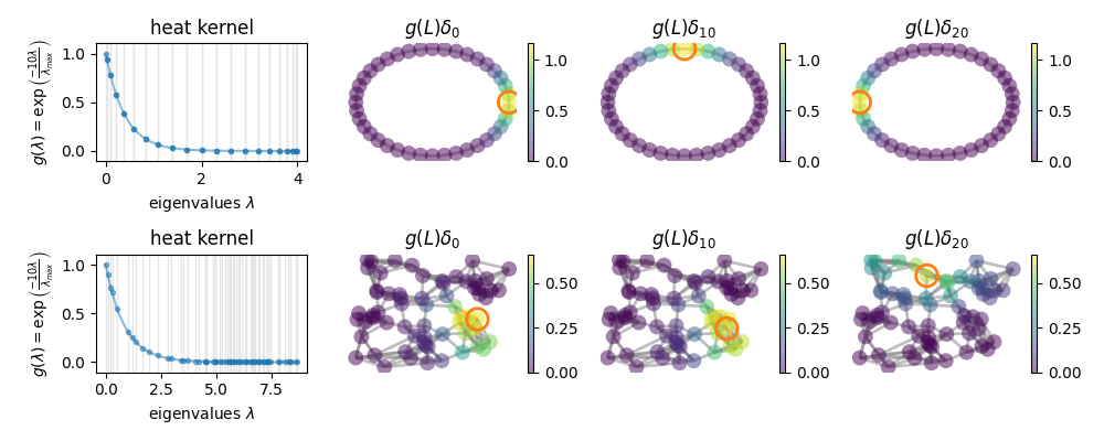
Kernel localization

In classical signal processing, a filter can be translated in the vertex domain. We cannot do that on graphs. Instead, we can localize() a filter kernel. Note how on classic structures (like the ring), the localized kernel is the same everywhere, while it changes when localized on irregular graphs.

import numpy as np
from matplotlib import pyplot as plt
import pygsp as pg

fig, axes = plt.subplots(2, 4, figsize=(10, 4))

graphs = [
    pg.graphs.Ring(40),
    pg.graphs.Sensor(64, seed=42),
]

locations = [0, 10, 20]

for graph, axs in zip(graphs, axes):
    graph.compute_fourier_basis()
    g = pg.filters.Heat(graph)
    g.plot(ax=axs[0], title='heat kernel')
    axs[0].set_xlabel(r'eigenvalues $\lambda$')
    axs[0].set_ylabel(r'$g(\lambda) = \exp \left( \frac{{-{}\lambda}}{{\lambda_{{max}}}} \right)$'.format(g.scale[0]))
    maximum = 0
    for loc in locations:
        x = g.localize(loc)
        maximum = np.maximum(maximum, x.max())
    for loc, ax in zip(locations, axs[1:]):
        graph.plot(g.localize(loc), limits=[0, maximum], highlight=loc, ax=ax,
                   title=r'$g(L) \delta_{{{}}}$'.format(loc))
        ax.set_axis_off()

fig.tight_layout()

Estimated memory usage: 25 MB