Graphs
The pygsp.graphs module implements the graph class hierarchy. A graph
object is either constructed from an adjacency matrix, or by instantiating one
of the built-in graph models.
Interface
The Graph base class allows to construct a graph object from any
adjacency matrix and provides a common interface to that object. Derived
classes then allows to instantiate various standard graph models.
Attributes
Matrix operators
Weighted adjacency matrix of the graph. |
|
Fourier basis (eigenvectors of the Laplacian). |
|
Differential operator (for gradient and divergence). |
Vectors
The degree (number of neighbors) of vertices. |
|
The weighted degree of vertices. |
|
Eigenvalues of the Laplacian (square of graph frequencies). |
Scalars
Largest eigenvalue of the graph Laplacian. |
|
Coherence of the Fourier basis. |
Attributes computation
|
Compute a graph Laplacian. |
|
Estimate the Laplacian's largest eigenvalue (cached). |
|
Compute the (partial) Fourier basis of the graph (cached). |
Compute the graph differential operator (cached). |
Differential operators
|
Compute the gradient of a signal defined on the vertices. |
|
Compute the divergence of a signal defined on the edges. |
Compute the Dirichlet energy of a signal defined on the vertices. |
Transforms
|
Compute the graph Fourier transform. |
|
Compute the inverse graph Fourier transform. |
Vertex-frequency transforms are implemented as filter banks and are found in
pygsp.filters (such as Gabor and
Modulation).
Checks
Check if the graph is weighted. |
|
Check if the graph is connected (cached). |
|
Check if the graph has directed edges (cached). |
|
Check if any vertex is connected to itself. |
Plotting
|
Plot a graph with signals as color or vertex size. |
|
Plot the graph's spectrogram. |
Import and export (I/O)
We provide import and export facility to two well-known Python packages for network analysis: NetworkX and graph-tool. Those packages and the PyGSP are fundamentally different in their goals (graph analysis versus graph signal analysis) and graph representations (if in the PyGSP everything is an ndarray, in NetworkX everything is a dictionary). Those tools are complementary and good interoperability is necessary to exploit the strengths of each tool. We ourselves leverage NetworkX and graph-tool to save and load graphs.
Note: to tie a signal with the graph, such that they are exported together,
attach it first with Graph.set_signal().
|
Load a graph from a file. |
|
Save the graph to a file. |
|
Import a graph from NetworkX. |
Export the graph to NetworkX. |
|
|
Import a graph from graph-tool. |
Export the graph to graph-tool. |
Others
Return an edge list, an alternative representation of the graph. |
|
|
Attach a signal to the graph. |
|
Set node's coordinates (their position when plotting). |
|
Create a subgraph from a list of vertices. |
Split the graph into connected components. |
Graph models
In addition to the below graphs, useful resources are the random graph
generators from NetworkX (see NetworkX’s documentation) and graph-tool (see
graph_tool.generation), as well as graph-tool’s assortment of standard
networks (see graph_tool.collection).
Any graph created by NetworkX or graph-tool can be imported in the PyGSP with
Graph.from_networkx() and Graph.from_graphtool().
Graphs built from other graphs
|
Build the line graph of a graph. |
Generated graphs
|
Airfoil graph. |
|
Barabasi-Albert preferential attachment. |
|
Comet graph. |
|
Community graph. |
|
Sensor network. |
|
Erdos Renyi graph. |
|
Fully connected graph. |
|
2-dimensional grid graph. |
|
GSP logo. |
|
Low stretch tree. |
|
Minnesota road network (from MatlabBGL). |
|
Path graph. |
|
Random k-regular graph. |
|
Ring graph with randomly sampled vertices. |
|
K-regular ring graph. |
|
Star graph. |
|
Stochastic Block Model (SBM). |
|
Sampled Swiss roll manifold. |
|
Sampled torus manifold. |
Nearest-neighbors graphs constructed from point clouds
|
Nearest-neighbor graph from given point cloud. |
|
Stanford bunny (NN-graph). |
|
Hyper-cube (NN-graph). |
|
NN-graph between patches of an image. |
|
Union of a patch graph with a 2D grid graph. |
|
Random sensor graph. |
|
Spherical-shaped graph (NN-graph). |
|
Two Moons (NN-graph). |
- class pygsp.graphs.Graph(adjacency, lap_type='combinatorial', coords=None, plotting={})[source]
Base graph class.
Instantiate it to construct a graph from a (weighted) adjacency matrix.
Provide a common interface (and implementation) for graph objects.
Initialize attributes for derived classes.
- Parameters:
- adjacencysparse matrix or array_like
The (weighted) adjacency matrix of size n_vertices by n_vertices that encodes the graph. The data is copied except if it is a sparse matrix in CSR format.
- lap_type{‘combinatorial’, ‘normalized’}
The kind of Laplacian to be computed by
compute_laplacian().- coordsarray_like
A matrix of size n_vertices by d that represents the coordinates of the vertices in a d-dimensional embedding space.
- plottingdict
Plotting parameters.
- Attributes:
- n_vertices or Nint
The number of vertices (nodes) in the graph.
- n_edges or Neint
The number of edges (links) in the graph.
Wscipy.sparse.csr_matrixWeighted adjacency matrix of the graph.
- L
scipy.sparse.csr_matrix The graph Laplacian, an N-by-N matrix computed from W.
- lap_type‘normalized’, ‘combinatorial’
The kind of Laplacian that was computed by
compute_laplacian().- signalsdict (string ->
numpy.ndarray) Signals attached to the graph.
- coords
numpy.ndarray Vertices coordinates in 2D or 3D space. Used for plotting only.
- plottingdict
Plotting parameters.
Examples
Define a simple graph.
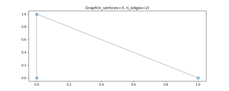
>>> graph = graphs.Graph([
...     [0., 2., 0.],
...     [2., 0., 5.],
...     [0., 5., 0.],
... ])
>>> graph
Graph(n_vertices=3, n_edges=2)
>>> graph.n_vertices, graph.n_edges
(3, 2)
>>> graph.W.toarray()
array([[0., 2., 0.],
       [2., 0., 5.],
       [0., 5., 0.]])
>>> graph.d
array([1, 2, 1], dtype=int32)
>>> graph.dw
array([2., 7., 5.])
>>> graph.L.toarray()
array([[ 2., -2.,  0.],
       [-2.,  7., -5.],
       [ 0., -5.,  5.]])
Add some coordinates to plot it.
>>> import matplotlib.pyplot as plt
>>> graph.set_coordinates([
...     [0, 0],
...     [0, 1],
...     [1, 0],
... ])
>>> fig, ax = graph.plot()
- classmethod from_graphtool(graph, weight='weight')
Import a graph from graph-tool.
Edge weights are retrieved as an edge property, under the name specified by the
weightparameter.Signals are retrieved from node properties, and stored in the
signalsdictionary under the property name. N-dimensional signals that were broken during export are joined.- Parameters:
- graph
graph_tool.Graph A graph-tool graph object.
- weightstring
The edge property that holds the numerical values used as the edge weights. All edge weights are set to 1 if None, or not found.
- graph
- Returns:
- graph
Graph A PyGSP graph object.
- graph
See also
from_networkximport from NetworkX
loadload from a file
Notes
If the graph has multiple edge connecting the same two nodes, a sum over the edges is taken to merge them.
Examples
>>> import graph_tool as gt
>>> graph = gt.Graph(directed=False)
>>> e1 = graph.add_edge(0, 1)
>>> e2 = graph.add_edge(1, 2)
>>> v = graph.add_vertex()
>>> eprop = graph.new_edge_property("double")
>>> eprop[e1] = 0.2
>>> eprop[graph.edge(1, 2)] = 0.9
>>> graph.edge_properties["weight"] = eprop
>>> vprop = graph.new_vertex_property("double", val=np.nan)
>>> vprop[3] = 3.1416
>>> graph.vertex_properties["sig"] = vprop
>>> graph = graphs.Graph.from_graphtool(graph)
>>> graph.W.toarray()
array([[0. , 0.2, 0. , 0. ],
       [0.2, 0. , 0.9, 0. ],
       [0. , 0.9, 0. , 0. ],
       [0. , 0. , 0. , 0. ]])
>>> graph.signals
{'sig': PropertyArray([   nan,    nan,    nan, 3.1416])}
- classmethod from_networkx(graph, weight='weight')
Import a graph from NetworkX.
Edge weights are retrieved as an edge attribute, under the name specified by the
weightparameter.Signals are retrieved from node attributes, and stored in the
signalsdictionary under the attribute name. N-dimensional signals that were broken during export are joined.- Parameters:
- graph
networkx.Graph A NetworkX graph object.
- weightstring or None, optional
The edge attribute that holds the numerical values used as the edge weights. All edge weights are set to 1 if None, or not found.
- graph
- Returns:
- graph
Graph A PyGSP graph object.
- graph
See also
from_graphtoolimport from graph-tool
loadload from a file
Notes
The nodes are ordered according to
networkx.Graph.nodes().In NetworkX, node attributes need not be set for every node. If a node attribute is not set for a node, a NaN is assigned to the corresponding signal for that node.
If the graph is a
networkx.MultiGraph, multiedges are aggregated by summation.Examples
>>> import networkx as nx
>>> graph = nx.Graph()
>>> graph.add_edge(1, 2, weight=0.2)
>>> graph.add_edge(2, 3, weight=0.9)
>>> graph.add_node(4, sig=3.1416)
>>> graph.nodes()
NodeView((1, 2, 3, 4))
>>> graph = graphs.Graph.from_networkx(graph)
>>> graph.W.toarray()
array([[0. , 0.2, 0. , 0. ],
       [0.2, 0. , 0.9, 0. ],
       [0. , 0.9, 0. , 0. ],
       [0. , 0. , 0. , 0. ]])
>>> graph.signals
{'sig': array([   nan,    nan,    nan, 3.1416])}
- classmethod load(path, fmt=None, backend=None)
Load a graph from a file.
Edge weights are retrieved as an edge attribute named “weight”.
Signals are retrieved from node attributes, and stored in the
signalsdictionary under the attribute name. N-dimensional signals that were broken during export are joined.- Parameters:
- pathstring
Path to the file from which to load the graph.
- fmt{‘graphml’, ‘gml’, ‘gexf’, None}, optional
Format in which the graph is saved. Guessed from the filename extension if None.
- backend{‘networkx’, ‘graph-tool’, None}, optional
Library used to load the graph. Automatically chosen if None.
- Returns:
- graph
Graph The loaded graph.
- graph
See also
savesave a graph to a file
from_networkxload with NetworkX then import in the PyGSP
from_graphtoolload with graph-tool then import in the PyGSP
Notes
A lossless round-trip is only guaranteed if the graph (and its signals) is saved and loaded with the same backend.
Loading from other formats is possible by loading in NetworkX or graph-tool, and importing to the PyGSP. The proposed formats are however tested for faithful round-trips.
Examples
>>> graph = graphs.Logo()
>>> graph.save('logo.graphml')
>>> graph = graphs.Graph.load('logo.graphml')
>>> import os
>>> os.remove('logo.graphml')
- compute_differential_operator()
Compute the graph differential operator (cached).
The differential operator is the matrix \(D\) such that
\[L = D D^\top,\]where \(L\) is the graph Laplacian (combinatorial or normalized). It is used to compute the gradient and the divergence of graph signals (see
grad()anddiv()).The differential operator computes the gradient and divergence of signals, and the Laplacian computes the divergence of the gradient, as follows:
\[z = L x = D y = D D^\top x,\]where \(y = D^\top x = \nabla_\mathcal{G} x\) is the gradient of \(x\) and \(z = D y = \operatorname{div}_\mathcal{G} y\) is the divergence of \(y\). See
grad()anddiv()for details.The difference operator is actually an incidence matrix of the graph, defined as
\[\begin{split}D[i, k] = \begin{cases} -\sqrt{W[i, j] / 2} & \text{if } e_k = (v_i, v_j) \text{ for some } j, \\ +\sqrt{W[i, j] / 2} & \text{if } e_k = (v_j, v_i) \text{ for some } j, \\ 0 & \text{otherwise} \end{cases}\end{split}\]for the combinatorial Laplacian, and
\[\begin{split}D[i, k] = \begin{cases} -\sqrt{W[i, j] / 2 / d[i]} & \text{if } e_k = (v_i, v_j) \text{ for some } j, \\ +\sqrt{W[i, j] / 2 / d[i]} & \text{if } e_k = (v_j, v_i) \text{ for some } j, \\ 0 & \text{otherwise} \end{cases}\end{split}\]for the normalized Laplacian, where \(v_i \in \mathcal{V}\) is a vertex, \(e_k = (v_i, v_j) \in \mathcal{E}\) is an edge from \(v_i\) to \(v_j\), \(W[i, j]\) is the weight
Wof the edge \((v_i, v_j)\), \(d[i]\) is the degreedwof vertex \(v_i\).For undirected graphs, only half the edges are kept (the upper triangular part of the adjacency matrix) in the interest of space and time. In that case, the \(1/\sqrt{2}\) factor disappears from the above equations for \(L = D D^\top\) to stand at all times.
The result is cached and accessible by the
Dproperty.Examples
The difference operator is an incidence matrix. Example with a undirected graph.
>>> graph = graphs.Graph([
...     [0, 2, 0],
...     [2, 0, 1],
...     [0, 1, 0],
... ])
>>> graph.compute_laplacian('combinatorial')
>>> graph.compute_differential_operator()
>>> graph.D.toarray()
array([[-1.41421356,  0.        ],
       [ 1.41421356, -1.        ],
       [ 0.        ,  1.        ]])
>>> graph.compute_laplacian('normalized')
>>> graph.compute_differential_operator()
>>> graph.D.toarray()
array([[-1.        ,  0.        ],
       [ 0.81649658, -0.57735027],
       [ 0.        ,  1.        ]])
Example with a directed graph.
>>> graph = graphs.Graph([
...     [0, 2, 0],
...     [2, 0, 1],
...     [0, 0, 0],
... ])
>>> graph.compute_laplacian('combinatorial')
>>> graph.compute_differential_operator()
>>> graph.D.toarray()
array([[-1.        ,  1.        ,  0.        ],
       [ 1.        , -1.        , -0.70710678],
       [ 0.        ,  0.        ,  0.70710678]])
>>> graph.compute_laplacian('normalized')
>>> graph.compute_differential_operator()
>>> graph.D.toarray()
array([[-0.70710678,  0.70710678,  0.        ],
       [ 0.63245553, -0.63245553, -0.4472136 ],
       [ 0.        ,  0.        ,  1.        ]])
The graph Laplacian acts on a signal as the divergence of the gradient.
>>> G = graphs.Logo()
>>> G.compute_differential_operator()
>>> s = np.random.default_rng().normal(size=G.N)
>>> s_grad = G.D.T.dot(s)
>>> s_lap = G.D.dot(s_grad)
>>> np.linalg.norm(s_lap - G.L.dot(s)) < 1e-10
True
- compute_fourier_basis(n_eigenvectors=None)
Compute the (partial) Fourier basis of the graph (cached).
The result is cached and accessible by the
U,e,lmax, andcoherenceproperties.- Parameters:
- n_eigenvectorsint or None
Number of eigenvectors to compute. If None, all eigenvectors are computed. (default: None)
Notes
‘G.compute_fourier_basis()’ computes a full eigendecomposition of the graph Laplacian \(L\) such that:
\[L = U \Lambda U^*,\]or a partial eigendecomposition of the graph Laplacian \(L\) such that:
\[L \approx U \Lambda U^*,\]where \(\Lambda\) is a diagonal matrix of eigenvalues and the columns of \(U\) are the eigenvectors.
G.e is a vector of length n_eigenvectors \(\le\) G.N containing the Laplacian eigenvalues. The largest eigenvalue is stored in G.lmax. The eigenvectors are stored as column vectors of G.U in the same order that the eigenvalues. Finally, the coherence of the Fourier basis is found in G.coherence.
References
See [Chu97].
Examples
>>> G = graphs.Torus()
>>> G.compute_fourier_basis(n_eigenvectors=64)
>>> G.U.shape
(256, 64)
>>> G.e.shape
(64,)
>>> G.compute_fourier_basis()
>>> G.U.shape
(256, 256)
>>> G.e.shape
(256,)
>>> G.lmax == G.e[-1]
True
>>> G.coherence < 1
True
- compute_laplacian(lap_type='combinatorial')[source]
Compute a graph Laplacian.
For undirected graphs, the combinatorial Laplacian is defined as
\[L = D - W,\]where \(W\) is the weighted adjacency matrix and \(D\) the weighted degree matrix. The normalized Laplacian is defined as
\[L = I - D^{-1/2} W D^{-1/2},\]where \(I\) is the identity matrix.
For directed graphs, the Laplacians are built from a symmetrized version of the weighted adjacency matrix that is the average of the weighted adjacency matrix and its transpose. As the Laplacian is defined as the divergence of the gradient, it is not affected by the orientation of the edges.
For both Laplacians, the diagonal entries corresponding to disconnected nodes (i.e., nodes with degree zero) are set to zero.
Once computed, the Laplacian is accessible by the attribute
L.- Parameters:
- lap_type{‘combinatorial’, ‘normalized’}
The kind of Laplacian to compute. Default is combinatorial.
Examples
Combinatorial and normalized Laplacians of an undirected graph.
>>> graph = graphs.Graph([
...     [0, 2, 0],
...     [2, 0, 1],
...     [0, 1, 0],
... ])
>>> graph.compute_laplacian('combinatorial')
>>> graph.L.toarray()
array([[ 2., -2.,  0.],
       [-2.,  3., -1.],
       [ 0., -1.,  1.]])
>>> graph.compute_laplacian('normalized')
>>> graph.L.toarray()
array([[ 1.        , -0.81649658,  0.        ],
       [-0.81649658,  1.        , -0.57735027],
       [ 0.        , -0.57735027,  1.        ]])
Combinatorial and normalized Laplacians of a directed graph.
>>> graph = graphs.Graph([
...     [0, 2, 0],
...     [2, 0, 1],
...     [0, 0, 0],
... ])
>>> graph.compute_laplacian('combinatorial')
>>> graph.L.toarray()
array([[ 2. , -2. ,  0. ],
       [-2. ,  2.5, -0.5],
       [ 0. , -0.5,  0.5]])
>>> graph.compute_laplacian('normalized')
>>> graph.L.toarray()
array([[ 1.        , -0.89442719,  0.        ],
       [-0.89442719,  1.        , -0.4472136 ],
       [ 0.        , -0.4472136 ,  1.        ]])
The Laplacian is defined as the divergence of the gradient. See
compute_differential_operator()for details.>>> graph = graphs.Path(20) >>> graph.compute_differential_operator() >>> L = graph.D.dot(graph.D.T) >>> np.all(L.toarray() == graph.L.toarray()) True
The Laplacians have a bounded spectrum.
>>> G = graphs.Sensor(50)
>>> G.compute_laplacian('combinatorial')
>>> G.compute_fourier_basis()
>>> -1e-10 < G.e[0] < 1e-10 < G.e[-1] < 2*np.max(G.dw)
True
>>> G.compute_laplacian('normalized')
>>> G.compute_fourier_basis()
>>> -1e-10 < G.e[0] < 1e-10 < G.e[-1] < 2
True
- dirichlet_energy(x)[source]
Compute the Dirichlet energy of a signal defined on the vertices.
The Dirichlet energy of a signal \(x\) is defined as
\[x^\top L x = \| \nabla_\mathcal{G} x \|_2^2 = \frac12 \sum_{i,j} W[i, j] (x[j] - x[i])^2\]for the combinatorial Laplacian, and
\[x^\top L x = \| \nabla_\mathcal{G} x \|_2^2 = \frac12 \sum_{i,j} W[i, j] \left( \frac{x[j]}{d[j]} - \frac{x[i]}{d[i]} \right)^2\]for the normalized Laplacian, where \(d\) is the weighted degree
dw, \(\nabla_\mathcal{G} x = D^\top x\) and \(D\) is the differential operatorD. Seegrad()for the definition of the gradient \(\nabla_\mathcal{G}\).- Parameters:
- xarray_like
Signal of length
n_verticesliving on the vertices.
- Returns:
- energyfloat
The Dirichlet energy of the graph signal.
See also
gradcompute the gradient of a vertex signal
Examples
Non-directed graph:
>>> graph = graphs.Path(5, directed=False)
>>> signal = [0, 2, 2, 4, 4]
>>> graph.dirichlet_energy(signal)
8.0
>>> # The Dirichlet energy is indeed the squared norm of the gradient.
>>> graph.compute_differential_operator()
>>> graph.grad(signal)
array([2., 0., 2., 0.])
Directed graph:
>>> graph = graphs.Path(5, directed=True)
>>> signal = [0, 2, 2, 4, 4]
>>> graph.dirichlet_energy(signal)
4.0
>>> # The Dirichlet energy is indeed the squared norm of the gradient.
>>> graph.compute_differential_operator()
>>> graph.grad(signal)
array([1.41421356, 0.        , 1.41421356, 0.        ])
- div(y)
Compute the divergence of a signal defined on the edges.
The divergence \(z\) of a signal \(y\) is defined as
\[z = \operatorname{div}_\mathcal{G} y = D y,\]where \(D\) is the differential operator
D.The value of the divergence on the vertex \(v_i\) is
\[z[i] = \sum_k D[i, k] y[k] = \sum_{\{k,j | e_k=(v_j, v_i) \in \mathcal{E}\}} \sqrt{\frac{W[j, i]}{2}} y[k] - \sum_{\{k,j | e_k=(v_i, v_j) \in \mathcal{E}\}} \sqrt{\frac{W[i, j]}{2}} y[k]\]for the combinatorial Laplacian, and
\[z[i] = \sum_k D[i, k] y[k] = \sum_{\{k,j | e_k=(v_j, v_i) \in \mathcal{E}\}} \sqrt{\frac{W[j, i]}{2 d[i]}} y[k] - \sum_{\{k,j | e_k=(v_i, v_j) \in \mathcal{E}\}} \sqrt{\frac{W[i, j]}{2 d[i]}} y[k]\]for the normalized Laplacian.
For undirected graphs, only half the edges are kept and the \(1/\sqrt{2}\) factor disappears from the above equations. See
compute_differential_operator()for details.- Parameters:
- yarray_like
Signal of length
n_edgesliving on the edges.
- Returns:
- zndarray
Divergence signal of length
n_verticesliving on the vertices.
See also
compute_differential_operatorgradcompute the gradient of a vertex signal
Examples
Non-directed graph and combinatorial Laplacian:
>>> graph = graphs.Path(4, directed=False, lap_type='combinatorial')
>>> graph.compute_differential_operator()
>>> graph.div([2, -2, 0])
array([-2.,  4., -2.,  0.])
Directed graph and combinatorial Laplacian:
>>> graph = graphs.Path(4, directed=True, lap_type='combinatorial')
>>> graph.compute_differential_operator()
>>> graph.div([2, -2, 0])
array([-1.41421356,  2.82842712, -1.41421356,  0.        ])
Non-directed graph and normalized Laplacian:
>>> graph = graphs.Path(4, directed=False, lap_type='normalized')
>>> graph.compute_differential_operator()
>>> graph.div([2, -2, 0])
array([-2.        ,  2.82842712, -1.41421356,  0.        ])
Directed graph and normalized Laplacian:
>>> graph = graphs.Path(4, directed=True, lap_type='normalized')
>>> graph.compute_differential_operator()
>>> graph.div([2, -2, 0])
array([-2.        ,  2.82842712, -1.41421356,  0.        ])
- estimate_lmax(method='lanczos')[source]
Estimate the Laplacian’s largest eigenvalue (cached).
The result is cached and accessible by the
lmaxproperty.Exact value given by the eigendecomposition of the Laplacian, see
compute_fourier_basis(). That estimation is much faster than the eigendecomposition.- Parameters:
- method{‘lanczos’, ‘bounds’}
Whether to estimate the largest eigenvalue with the implicitly restarted Lanczos method, or to return an upper bound on the spectrum of the Laplacian.
Notes
Runs the implicitly restarted Lanczos method (as implemented in
scipy.sparse.linalg.eigsh()) with a large tolerance, then increases the calculated largest eigenvalue by 1 percent. For much of the PyGSP machinery, we need to approximate filter kernels on an interval that contains the spectrum of L. The only cost of using a larger interval is that the polynomial approximation over the larger interval may be a slightly worse approximation on the actual spectrum. As this is a very mild effect, it is not necessary to obtain very tight bounds on the spectrum of L.A faster but less tight alternative is to use known algebraic bounds on the graph Laplacian.
Examples
>>> G = graphs.Logo()
>>> G.compute_fourier_basis()  # True value.
>>> print('{:.2f}'.format(G.lmax))
13.78
>>> G.estimate_lmax(method='lanczos')  # Estimate.
>>> print('{:.2f}'.format(G.lmax))
13.92
>>> G.estimate_lmax(method='bounds')  # Upper bound.
>>> print('{:.2f}'.format(G.lmax))
18.58
- extract_components()[source]
Split the graph into connected components.
See
is_connected()for the method used to determine connectedness.- Returns:
- graphslist
A list of graph structures. Each having its own node list and weight matrix. If the graph is directed, add into the info parameter the information about the source nodes and the sink nodes.
Examples
>>> from scipy import sparse
>>> W = sparse.rand(10, 10, 0.2)
>>> W = utils.symmetrize(W)
>>> G = graphs.Graph(W)
>>> components = G.extract_components()
>>> has_sinks = 'sink' in components[0].info
>>> sinks_0 = components[0].info['sink'] if has_sinks else []
- get_edge_list()[source]
Return an edge list, an alternative representation of the graph.
Each edge \(e_k = (v_i, v_j) \in \mathcal{E}\) from \(v_i\) to \(v_j\) is associated with the weight \(W[i, j]\). For each edge \(e_k\), the method returns \((i, j, W[i, j])\) as (sources[k], targets[k], weights[k]), with \(i \in [0, |\mathcal{V}|-1], j \in [0, |\mathcal{V}|-1], k \in [0, |\mathcal{E}|-1]\).
- Returns:
- sourcesvector of int
Source node indices.
- targetsvector of int
Target node indices.
- weightsvector of float
Edge weights.
Notes
The weighted adjacency matrix is the canonical form used in this package to represent a graph as it is the easiest to work with when considering spectral methods.
Edge orientation (i.e., which node is the source or the target) is arbitrary for undirected graphs. The implementation uses the upper triangular part of the adjacency matrix, hence \(i \leq j \ \forall k\).
Examples
Edge list of a directed graph.
>>> graph = graphs.Graph([
...     [0, 3, 0],
...     [3, 0, 4],
...     [0, 0, 0],
... ])
>>> sources, targets, weights = graph.get_edge_list()
>>> list(sources), list(targets), list(weights)
([0, 1, 1], [1, 0, 2], [3, 3, 4])
Edge list of an undirected graph.
>>> graph = graphs.Graph([
...     [0, 3, 0],
...     [3, 0, 4],
...     [0, 4, 0],
... ])
>>> sources, targets, weights = graph.get_edge_list()
>>> list(sources), list(targets), list(weights)
([0, 1], [1, 2], [3, 4])
- gft(s)
Compute the graph Fourier transform.
The graph Fourier transform of a signal \(s\) is defined as
\[\hat{s} = U^* s,\]where \(U\) is the Fourier basis attr:U and \(U^*\) denotes the conjugate transpose or Hermitian transpose of \(U\).
- Parameters:
- sarray_like
Graph signal in the vertex domain.
- Returns:
- s_hatndarray
Representation of s in the Fourier domain.
Examples
>>> G = graphs.Logo()
>>> G.compute_fourier_basis()
>>> s = np.random.default_rng().normal(size=(G.N, 5, 1))
>>> s_hat = G.gft(s)
>>> s_star = G.igft(s_hat)
>>> np.all((s - s_star) < 1e-10)
True
- grad(x)
Compute the gradient of a signal defined on the vertices.
The gradient \(y\) of a signal \(x\) is defined as
\[y = \nabla_\mathcal{G} x = D^\top x,\]where \(D\) is the differential operator
D.The value of the gradient on the edge \(e_k = (v_i, v_j)\) from \(v_i\) to \(v_j\) with weight \(W[i, j]\) is
\[y[k] = D[i, k] x[i] + D[j, k] x[j] = \sqrt{\frac{W[i, j]}{2}} (x[j] - x[i])\]for the combinatorial Laplacian, and
\[y[k] = \sqrt{\frac{W[i, j]}{2}} \left( \frac{x[j]}{\sqrt{d[j]}} - \frac{x[i]}{\sqrt{d[i]}} \right)\]for the normalized Laplacian.
For undirected graphs, only half the edges are kept and the \(1/\sqrt{2}\) factor disappears from the above equations. See
compute_differential_operator()for details.- Parameters:
- xarray_like
Signal of length
n_verticesliving on the vertices.
- Returns:
- yndarray
Gradient signal of length
n_edgesliving on the edges.
See also
compute_differential_operatordivcompute the divergence of an edge signal
dirichlet_energycompute the norm of the gradient
Examples
Non-directed graph and combinatorial Laplacian:
>>> graph = graphs.Path(4, directed=False, lap_type='combinatorial')
>>> graph.compute_differential_operator()
>>> graph.grad([0, 2, 4, 2])
array([ 2.,  2., -2.])
Directed graph and combinatorial Laplacian:
>>> graph = graphs.Path(4, directed=True, lap_type='combinatorial')
>>> graph.compute_differential_operator()
>>> graph.grad([0, 2, 4, 2])
array([ 1.41421356,  1.41421356, -1.41421356])
Non-directed graph and normalized Laplacian:
>>> graph = graphs.Path(4, directed=False, lap_type='normalized')
>>> graph.compute_differential_operator()
>>> graph.grad([0, 2, 4, 2])
array([ 1.41421356,  1.41421356, -0.82842712])
Directed graph and normalized Laplacian:
>>> graph = graphs.Path(4, directed=True, lap_type='normalized')
>>> graph.compute_differential_operator()
>>> graph.grad([0, 2, 4, 2])
array([ 1.41421356,  1.41421356, -0.82842712])
- has_loops()[source]
Check if any vertex is connected to itself.
A graph has self-loops if and only if the diagonal entries of its adjacency matrix are not all zero.
- Returns:
- loopsbool
True if the graph has self-loops, False otherwise.
Examples
Without self-loops:
>>> graph = graphs.Graph([
...     [0, 3, 0],
...     [3, 0, 4],
...     [0, 0, 0],
... ])
>>> graph.has_loops()
False
With a self-loop:
>>> graph = graphs.Graph([
...     [1, 3, 0],
...     [3, 0, 4],
...     [0, 0, 0],
... ])
>>> graph.has_loops()
True
- igft(s_hat)
Compute the inverse graph Fourier transform.
The inverse graph Fourier transform of a Fourier domain signal \(\hat{s}\) is defined as
\[s = U \hat{s},\]where \(U\) is the Fourier basis
U.- Parameters:
- s_hatarray_like
Graph signal in the Fourier domain.
- Returns:
- sndarray
Representation of s_hat in the vertex domain.
Examples
>>> G = graphs.Logo()
>>> G.compute_fourier_basis()
>>> s_hat = np.random.default_rng().normal(size=(G.N, 5, 1))
>>> s = G.igft(s_hat)
>>> s_hat_star = G.gft(s)
>>> np.all((s_hat - s_hat_star) < 1e-10)
True
- is_connected()[source]
Check if the graph is connected (cached).
A graph is connected if and only if there exists a (directed) path between any two vertices.
- Returns:
- connectedbool
True if the graph is connected, False otherwise.
Notes
For undirected graphs, starting at a vertex and trying to visit all the others is enough. For directed graphs, one needs to check that a vertex can both be visited by all the others and visit all the others.
Examples
Connected graph:
>>> graph = graphs.Graph([
...     [0, 3, 0, 0],
...     [3, 0, 4, 0],
...     [0, 4, 0, 2],
...     [0, 0, 2, 0],
... ])
>>> graph.is_connected()
True
Disconnected graph:
>>> graph = graphs.Graph([
...     [0, 3, 0, 0],
...     [3, 0, 4, 0],
...     [0, 0, 0, 2],
...     [0, 0, 2, 0],
... ])
>>> graph.is_connected()
False
- is_directed()[source]
Check if the graph has directed edges (cached).
In this framework, we consider that a graph is directed if and only if its weight matrix is not symmetric.
- Returns:
- directedbool
True if the graph is directed, False otherwise.
Examples
Directed graph:
>>> graph = graphs.Graph([
...     [0, 3, 0],
...     [3, 0, 4],
...     [0, 0, 0],
... ])
>>> graph.is_directed()
True
Undirected graph:
>>> graph = graphs.Graph([
...     [0, 3, 0],
...     [3, 0, 4],
...     [0, 4, 0],
... ])
>>> graph.is_directed()
False
- is_weighted()[source]
Check if the graph is weighted.
A graph is unweighted (binary) if and only if all the entries in the adjacency matrix are either zero or one.
- Returns:
- weightedbool
True if the graph is weighted, False otherwise.
Examples
Unweighted (binary) graph:
>>> graph = graphs.Graph([
...     [0, 1, 0],
...     [1, 0, 1],
...     [0, 1, 0],
... ])
>>> graph.is_weighted()
False
Weighted graph:
>>> graph = graphs.Graph([
...     [0, 2, 0],
...     [2, 0, 1],
...     [0, 1, 0],
... ])
>>> graph.is_weighted()
True
- plot(vertex_color=None, vertex_size=None, highlight=[], edges=None, edge_color=None, edge_width=None, indices=False, colorbar=True, limits=None, ax=None, title=None, backend=None)[source]
Plot a graph with signals as color or vertex size.
- Parameters:
- vertex_colorarray_like or color
Signal to plot as vertex color (length is the number of vertices). If None, vertex color is set to graph.plotting[‘vertex_color’]. Alternatively, a color can be set in any format accepted by matplotlib. Each vertex color can by specified by an RGB(A) array of dimension n_vertices x 3 (or 4).
- vertex_sizearray_like or int
Signal to plot as vertex size (length is the number of vertices). Vertex size ranges from 0.5 to 2 times graph.plotting[‘vertex_size’]. If None, vertex size is set to graph.plotting[‘vertex_size’]. Alternatively, a size can be passed as an integer. The pyqtgraph backend only accepts an integer size.
- highlightiterable
List of indices of vertices to be highlighted. Useful for example to show where a filter was localized. Only available with the matplotlib backend.
- edgesbool
Whether to draw edges in addition to vertices. Default to True if less than 10,000 edges to draw. Note that drawing many edges can be slow.
- edge_colorarray_like or color
Signal to plot as edge color (length is the number of edges). Edge color is given by graph.plotting[‘edge_color’] and transparency ranges from 0.2 to 0.9. If None, edge color is set to graph.plotting[‘edge_color’]. Alternatively, a color can be set in any format accepted by matplotlib. Each edge color can by specified by an RGB(A) array of dimension n_edges x 3 (or 4). Only available with the matplotlib backend.
- edge_widtharray_like or int
Signal to plot as edge width (length is the number of edges). Edge width ranges from 0.5 to 2 times graph.plotting[‘edge_width’]. If None, edge width is set to graph.plotting[‘edge_width’]. Alternatively, a width can be passed as an integer. Only available with the matplotlib backend.
- indicesbool
Whether to print the node indices (in the adjacency / Laplacian matrix and signal vectors) on top of each node. Useful to locate a node of interest. Only available with the matplotlib backend.
- colorbarbool
Whether to plot a colorbar indicating the signal’s amplitude. Only available with the matplotlib backend.
- limits[vmin, vmax]
Map colors from vmin to vmax. Defaults to signal minimum and maximum value. Only available with the matplotlib backend.
- ax
matplotlib.axes.Axes Axes where to draw the graph. Optional, created if not passed. Only available with the matplotlib backend.
- titlestr
Title of the figure.
- backend: {‘matplotlib’, ‘pyqtgraph’, None}
Defines the drawing backend to use. Defaults to
pygsp.plotting.BACKEND.
- Returns:
- fig
matplotlib.figure.Figure The figure the plot belongs to. Only with the matplotlib backend.
- ax
matplotlib.axes.Axes The axes the plot belongs to. Only with the matplotlib backend.
- fig
Notes
The orientation of directed edges is not shown. If edges exist in both directions, they will be drawn on top of each other.
Examples
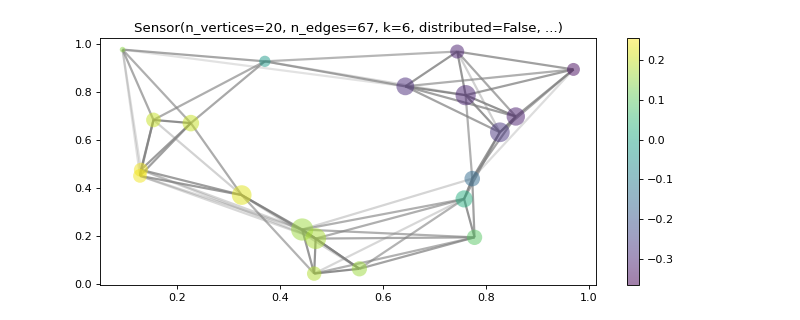
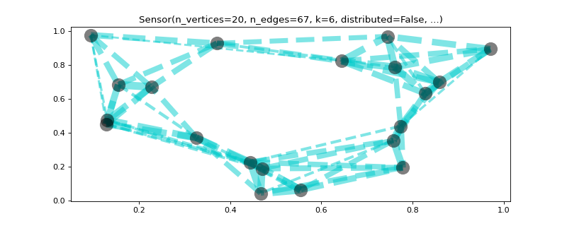
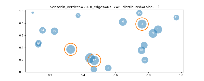
>>> import matplotlib
>>> graph = graphs.Sensor(20, seed=42)
>>> graph.compute_fourier_basis(n_eigenvectors=4)
>>> _, _, weights = graph.get_edge_list()
>>> fig, ax = graph.plot(graph.U[:, 1], vertex_size=graph.dw,
...                      edge_color=weights)
>>> graph.plotting['vertex_size'] = 300
>>> graph.plotting['edge_width'] = 5
>>> graph.plotting['edge_style'] = '--'
>>> fig, ax = graph.plot(edge_width=weights, edge_color=(0, .8, .8, .5),
...                      vertex_color='black')
>>> fig, ax = graph.plot(vertex_size=graph.dw, indices=True,
...                      highlight=[17, 3, 16], edges=False)
- plot_spectrogram(node_idx=None)[source]
Plot the graph’s spectrogram.
- Parameters:
- node_idxndarray
Order to sort the nodes in the spectrogram. By default, does not reorder the nodes.
Notes
This function is only implemented for the pyqtgraph backend at the moment.
Examples
>>> G = graphs.Ring(15)
>>> G.plot_spectrogram()
- save(path, fmt=None, backend=None)
Save the graph to a file.
Edge weights are stored as an edge attribute, under the name “weight”.
Signals are stored as node attributes, under their name in the
signalsdictionary. N-dimensional signals are broken into N 1-dimensional signals. They will eventually be joined back together on import.Supported formats are:
GraphML, a comprehensive XML format. Supported by NetworkX, graph-tool, NetworKit, igraph, Gephi, Cytoscape, SocNetV.
GML (Graph Modelling Language), a simple non-XML format. Supported by NetworkX, graph-tool, NetworKit, igraph, Gephi, Cytoscape, SocNetV, Tulip.
GEXF (Graph Exchange XML Format), Gephi’s XML format. Supported by NetworkX, NetworKit, Gephi, Tulip, ngraph.
If unsure, we recommend GraphML.
- Parameters:
- pathstring
Path to the file where the graph is to be saved.
- fmt{‘graphml’, ‘gml’, ‘gexf’, None}, optional
Format in which to save the graph. Guessed from the filename extension if None.
- backend{‘networkx’, ‘graph-tool’, None}, optional
Library used to load the graph. Automatically chosen if None.
See also
loadload a graph from a file
to_networkxexport as a NetworkX graph, and save with NetworkX
to_graphtoolexport as a graph-tool graph, and save with graph-tool
Notes
A lossless round-trip is only guaranteed if the graph (and its signals) is saved and loaded with the same backend.
Saving in other formats is possible by exporting to NetworkX or graph-tool, and using their respective saving functionality. The proposed formats are however tested for faithful round-trips.
Edge weights and signal values are rounded at the sixth decimal when saving in
fmt='gml'withbackend='graph-tool'.Examples
>>> graph = graphs.Logo()
>>> graph.save('logo.graphml')
>>> graph = graphs.Graph.load('logo.graphml')
>>> import os
>>> os.remove('logo.graphml')
- set_coordinates(kind='spring', seed=None, **kwargs)
Set node’s coordinates (their position when plotting).
- Parameters:
- kindstring or array_like
Kind of coordinates to generate. It controls the position of the nodes when plotting the graph. Can either pass an array of size Nx2 or Nx3 to set the coordinates manually or the name of a layout algorithm. Available algorithms: community2D, random2D, random3D, ring2D, line1D, spring, laplacian_eigenmap2D, laplacian_eigenmap3D. Default is ‘spring’.
- seedint
Seed for the random number generator when kind is ‘random’, ‘community’, or ‘spring’.
- kwargsdict
Additional parameters to be passed to the Fruchterman-Reingold force-directed algorithm when kind is spring.
Examples
>>> G = graphs.ErdosRenyi()
>>> G.set_coordinates()
>>> fig, ax = G.plot()
- set_signal(signal, name)[source]
Attach a signal to the graph.
Attached signals can be accessed (and modified or deleted) through the
signalsdictionary.- Parameters:
- signalarray_like
A sequence that assigns a value to each vertex. The value of the signal at vertex i is
signal[i].- nameString
Name of the signal used as a key in the
signalsdictionary.
Examples
>>> graph = graphs.Sensor(10)
>>> signal = np.arange(graph.n_vertices)
>>> graph.set_signal(signal, 'mysignal')
>>> graph.signals
{'mysignal': array([0, 1, 2, 3, 4, 5, 6, 7, 8, 9])}
- subgraph(vertices)[source]
Create a subgraph from a list of vertices.
- Parameters:
- verticeslist
Vertices to keep. Either a list of indices or an indicator function.
- Returns:
- subgraph
Graph Subgraph.
- subgraph
Examples
>>> graph = graphs.Graph([
...     [0., 3., 0., 0.],
...     [3., 0., 4., 0.],
...     [0., 4., 0., 2.],
...     [0., 0., 2., 0.],
... ])
>>> graph = graph.subgraph([0, 2, 1])
>>> graph.W.toarray()
array([[0., 0., 3.],
       [0., 0., 4.],
       [3., 4., 0.]])
- to_graphtool()
Export the graph to graph-tool.
Edge weights are stored as an edge property map, under the name “weight”.
Signals are stored as vertex property maps, under their name in the
signalsdictionary. N-dimensional signals are broken into N 1-dimensional signals. They will eventually be joined back together on import.- Returns:
- graph
graph_tool.Graph A graph-tool graph object.
- graph
See also
to_networkxexport to NetworkX
savesave to a file
Examples
>>> import graph_tool as gt
>>> import graph_tool.draw
>>> from matplotlib import pyplot as plt
>>> graph = graphs.Path(4, directed=True)
>>> graph.set_signal(np.full(4, 2.3), 'signal')
>>> graph = graph.to_graphtool()
>>> graph.is_directed()
True
>>> graph.vertex_properties['signal'][2]
2.3
>>> graph.edge_properties['weight'][graph.edge(0, 1)]
1.0
>>> # gt.draw.graph_draw(graph, vertex_text=graph.vertex_index)
Another common goal is to use graph-tool to compute some properties to be imported back in the PyGSP as signals.
>>> import graph_tool as gt
>>> import graph_tool.centrality
>>> from matplotlib import pyplot as plt
>>> graph = graphs.Sensor(100, seed=42)
>>> graph.set_signal(graph.coords, 'coords')
>>> graph = graph.to_graphtool()
>>> vprop, eprop = gt.centrality.betweenness(
...     graph, weight=graph.edge_properties['weight'])
>>> graph.vertex_properties['betweenness'] = vprop
>>> graph = graphs.Graph.from_graphtool(graph)
>>> graph.compute_fourier_basis()
>>> graph.set_coordinates(graph.signals['coords'])
>>> fig, axes = plt.subplots(1, 2)
>>> _ = graph.plot(graph.signals['betweenness'], ax=axes[0])
>>> _ = axes[1].plot(graph.e, graph.gft(graph.signals['betweenness']))
- to_networkx()
Export the graph to NetworkX.
Edge weights are stored as an edge attribute, under the name “weight”.
Signals are stored as node attributes, under their name in the
signalsdictionary. N-dimensional signals are broken into N 1-dimensional signals. They will eventually be joined back together on import.- Returns:
- graph
networkx.Graph A NetworkX graph object.
- graph
See also
to_graphtoolexport to graph-tool
savesave to a file
Examples
>>> import networkx as nx
>>> from matplotlib import pyplot as plt
>>> graph = graphs.Path(4, directed=True)
>>> graph.set_signal(np.full(4, 2.3), 'signal')
>>> graph = graph.to_networkx()
>>> print(nx.info(graph))
DiGraph named 'Path' with 4 nodes and 3 edges
>>> nx.is_directed(graph)
True
>>> graph.nodes()
NodeView((0, 1, 2, 3))
>>> graph.edges()
OutEdgeView([(0, 1), (1, 2), (2, 3)])
>>> graph.nodes()[2]
{'signal': 2.3}
>>> graph.edges()[(0, 1)]
{'weight': 1.0}
>>> # nx.draw(graph, with_labels=True)
Another common goal is to use NetworkX to compute some properties to be be imported back in the PyGSP as signals.
>>> import networkx as nx
>>> from matplotlib import pyplot as plt
>>> graph = graphs.Sensor(100, seed=42)
>>> graph.set_signal(graph.coords, 'coords')
>>> graph = graph.to_networkx()
>>> betweenness = nx.betweenness_centrality(graph, weight='weight')
>>> nx.set_node_attributes(graph, betweenness, 'betweenness')
>>> graph = graphs.Graph.from_networkx(graph)
>>> graph.compute_fourier_basis()
>>> graph.set_coordinates(graph.signals['coords'])
>>> fig, axes = plt.subplots(1, 2)
>>> _ = graph.plot(graph.signals['betweenness'], ax=axes[0])
>>> _ = axes[1].plot(graph.e, graph.gft(graph.signals['betweenness']))
- property A
Graph adjacency matrix (the binary version of W).
The adjacency matrix defines which edges exist on the graph. It is represented as an N-by-N matrix of booleans. \(A_{i,j}\) is True if \(W_{i,j} > 0\).
- property D
Differential operator (for gradient and divergence).
Is computed by
compute_differential_operator().
- property U
Fourier basis (eigenvectors of the Laplacian).
Is computed by
compute_fourier_basis().
- property W
Weighted adjacency matrix of the graph.
- property coherence
Coherence of the Fourier basis.
The mutual coherence between the basis of Kronecker deltas and the basis formed by the eigenvectors of the graph Laplacian is defined as
\[\mu = \max_{\ell,i} \langle U_\ell, \delta_i \rangle = \max_{\ell,i} | U_{\ell, i} | \in \left[ \frac{1}{\sqrt{N}}, 1 \right],\]where \(N\) is the number of vertices, \(\delta_i \in \mathbb{R}^N\) denotes the Kronecker delta that is non-zero on vertex \(v_i\), and \(U_\ell \in \mathbb{R}^N\) denotes the \(\ell^\text{th}\) eigenvector of the graph Laplacian (i.e., the \(\ell^\text{th}\) Fourier mode).
The coherence is a measure of the localization of the Fourier modes (Laplacian eigenvectors). The larger the value, the more localized the eigenvectors can be. The extreme is a node that is disconnected from the rest of the graph: an eigenvector will be localized as a Kronecker delta there (i.e., \(\mu = 1\)). In the classical setting, Fourier modes (which are complex exponentials) are completely delocalized, and the coherence is minimal.
The value is computed by
compute_fourier_basis().Examples
Delocalized eigenvectors.
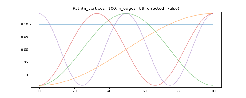
>>> graph = graphs.Path(100)
>>> graph.compute_fourier_basis()
>>> minimum = 1 / np.sqrt(graph.n_vertices)
>>> print('{:.2f} in [{:.2f}, 1]'.format(graph.coherence, minimum))
0.14 in [0.10, 1]
>>>
>>> # Plot some delocalized eigenvectors.
>>> import matplotlib.pyplot as plt
>>> graph.set_coordinates('line1D')
>>> _ = graph.plot(graph.U[:, :5])
Localized eigenvectors.
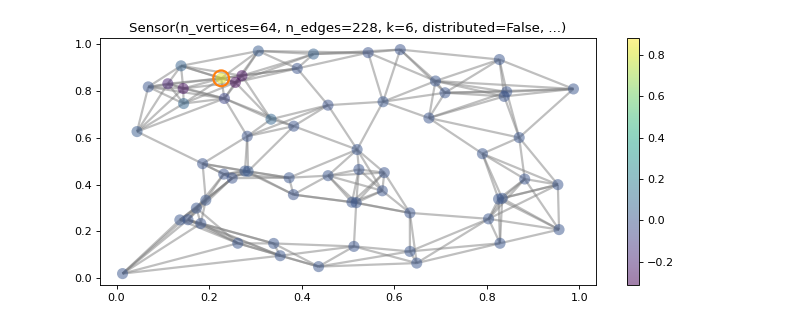
>>> graph = graphs.Sensor(64, seed=10)
>>> graph.compute_fourier_basis()
>>> minimum = 1 / np.sqrt(graph.n_vertices)
>>> print('{:.2f} in [{:.2f}, 1]'.format(graph.coherence, minimum))
0.84 in [0.12, 1]
>>>
>>> # Plot the most localized eigenvector.
>>> import matplotlib.pyplot as plt
>>> idx = np.argmax(np.abs(graph.U))
>>> idx_vertex, idx_fourier = np.unravel_index(idx, graph.U.shape)
>>> _ = graph.plot(graph.U[:, idx_fourier], highlight=idx_vertex)
- property d
The degree (number of neighbors) of vertices.
For undirected graphs, the degree of a vertex is the number of vertices it is connected to. For directed graphs, the degree is the average of the in and out degrees, where the in degree is the number of incoming edges, and the out degree the number of outgoing edges.
In both cases, the degree of the vertex \(v_i\) is the average between the number of non-zero values in the \(i\)-th column (the in degree) and the \(i\)-th row (the out degree) of the weighted adjacency matrix
W.Examples
Undirected graph:
>>> graph = graphs.Graph([
...     [0, 1, 0],
...     [1, 0, 2],
...     [0, 2, 0],
... ])
>>> print(graph.d)  # Number of neighbors.
[1 2 1]
>>> print(graph.dw)  # Weighted degree.
[1 3 2]
Directed graph:
>>> graph = graphs.Graph([
...     [0, 1, 0],
...     [0, 0, 2],
...     [0, 2, 0],
... ])
>>> print(graph.d)  # Number of neighbors.
[0.5 1.5 1. ]
>>> print(graph.dw)  # Weighted degree.
[0.5 2.5 2. ]
- property dw
The weighted degree of vertices.
For undirected graphs, the weighted degree of the vertex \(v_i\) is defined as
\[d[i] = \sum_j W[j, i] = \sum_j W[i, j],\]where \(W\) is the weighted adjacency matrix
W.For directed graphs, the weighted degree of the vertex \(v_i\) is defined as
\[d[i] = \frac12 (d^\text{in}[i] + d^\text{out}[i]) = \frac12 (\sum_j W[j, i] + \sum_j W[i, j]),\]i.e., as the average of the in and out degrees.
Examples
Undirected graph:
>>> graph = graphs.Graph([
...     [0, 1, 0],
...     [1, 0, 2],
...     [0, 2, 0],
... ])
>>> print(graph.d)  # Number of neighbors.
[1 2 1]
>>> print(graph.dw)  # Weighted degree.
[1 3 2]
Directed graph:
>>> graph = graphs.Graph([
...     [0, 1, 0],
...     [0, 0, 2],
...     [0, 2, 0],
... ])
>>> print(graph.d)  # Number of neighbors.
[0.5 1.5 1. ]
>>> print(graph.dw)  # Weighted degree.
[0.5 2.5 2. ]
- property e
Eigenvalues of the Laplacian (square of graph frequencies).
Is computed by
compute_fourier_basis().
- property lmax
Largest eigenvalue of the graph Laplacian.
Can be exactly computed by
compute_fourier_basis()or approximated byestimate_lmax().