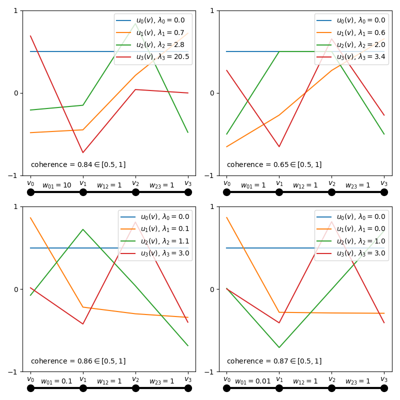
Localization of Fourier modes

The Fourier modes (the eigenvectors of the graph Laplacian) can be localized in the spacial domain. As a consequence, graph signals can be localized in both space and frequency (which is impossible for Euclidean domains or manifolds, by the Heisenberg’s uncertainty principle).

This example demonstrates that the more isolated a node is, the more a Fourier mode will be localized on it.

The mutual coherence between the basis of Kronecker deltas and the basis formed by the eigenvectors of the Laplacian, pygsp.graphs.Graph.coherence, is a measure of the localization of the Fourier modes. The larger the value, the more localized the eigenvectors can be.

See Global and Local Uncertainty Principles for Signals on Graphs for details.

import numpy as np
import matplotlib as mpl
from matplotlib import pyplot as plt
import pygsp as pg

fig, axes = plt.subplots(2, 2, figsize=(8, 8))

for w, ax in zip([10, 1, 0.1, 0.01], axes.flatten()):

    adjacency = [
        [0, w, 0, 0],
        [w, 0, 1, 0],
        [0, 1, 0, 1],
        [0, 0, 1, 0],
    ]
    graph = pg.graphs.Graph(adjacency)
    graph.compute_fourier_basis()

    # Plot eigenvectors.
    ax.plot(graph.U)
    ax.set_ylim(-1, 1)
    ax.set_yticks([-1, 0, 1])
    ax.legend([f'$u_{i}(v)$, $\lambda_{i}={graph.e[i]:.1f}$' for i in
              range(graph.n_vertices)], loc='upper right')

    ax.text(0, -0.9, f'coherence = {graph.coherence:.2f}'
            f'$\in [{1/np.sqrt(graph.n_vertices)}, 1]$')

    # Plot vertices.
    ax.set_xticks(range(graph.n_vertices))
    ax.set_xticklabels([f'$v_{i}$' for i in range(graph.n_vertices)])

    # Plot graph.
    x, y = np.arange(0, graph.n_vertices), -1.20*np.ones(graph.n_vertices)
    line = mpl.lines.Line2D(x, y, lw=3, color='k', marker='.', markersize=20)
    line.set_clip_on(False)
    ax.add_line(line)

    # Plot edge weights.
    for i in range(graph.n_vertices - 1):
        j = i+1
        ax.text(i+0.5, -1.15, f'$w_{{{i}{j}}} = {adjacency[i][j]}$',
                horizontalalignment='center')

fig.tight_layout()

Estimated memory usage: 9 MB