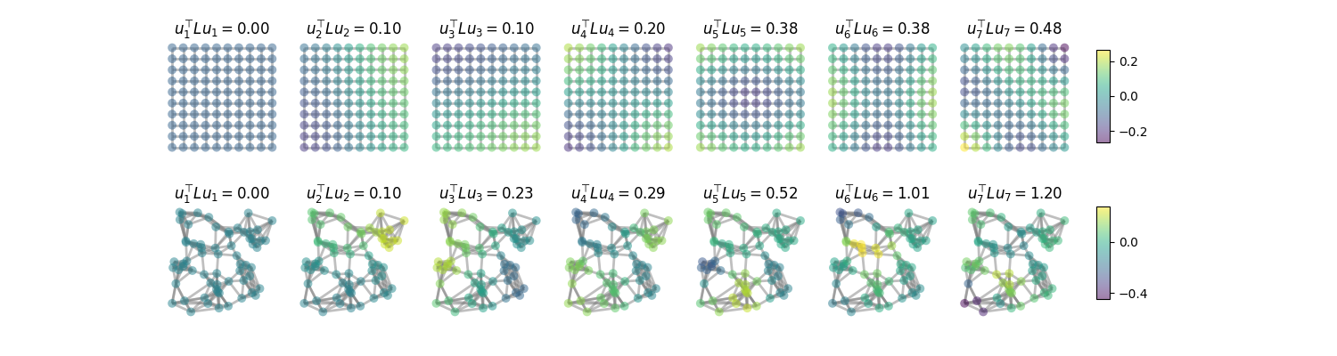
Fourier basis¶

The eigenvectors of the graph Laplacian form the Fourier basis. The eigenvalues are a measure of variation of their corresponding eigenvector. The lower the eigenvalue, the smoother the eigenvector. They are hence a measure of “frequency”.

In classical signal processing, Fourier modes are completely delocalized, like on the grid graph. For general graphs however, Fourier modes might be localized. See pygsp.graphs.Graph.coherence.

$u_1^\top L u_1 = 0.00$, $u_2^\top L u_2 = 0.10$, $u_3^\top L u_3 = 0.10$, $u_4^\top L u_4 = 0.20$, $u_5^\top L u_5 = 0.38$, $u_6^\top L u_6 = 0.38$, $u_7^\top L u_7 = 0.48$, $u_1^\top L u_1 = 0.00$, $u_2^\top L u_2 = 0.10$, $u_3^\top L u_3 = 0.23$, $u_4^\top L u_4 = 0.29$, $u_5^\top L u_5 = 0.52$, $u_6^\top L u_6 = 1.01$, $u_7^\top L u_7 = 1.20$

import numpy as np
from matplotlib import pyplot as plt
import pygsp as pg

n_eigenvectors = 7

fig, axes = plt.subplots(2, 7, figsize=(15, 4))

def plot_eigenvectors(G, axes):
    G.compute_fourier_basis(n_eigenvectors)
    limits = [f(G.U) for f in (np.min, np.max)]
    for i, ax in enumerate(axes):
        G.plot(G.U[:, i], limits=limits, colorbar=False, vertex_size=50, ax=ax)
        energy = abs(G.dirichlet_energy(G.U[:, i]))
        ax.set_title(r'$u_{0}^\top L u_{0} = {1:.2f}$'.format(i+1, energy))
        ax.set_axis_off()

G = pg.graphs.Grid2d(10, 10)
plot_eigenvectors(G, axes[0])
fig.subplots_adjust(hspace=0.5, right=0.8)
cax = fig.add_axes([0.82, 0.60, 0.01, 0.26])
fig.colorbar(axes[0, -1].collections[1], cax=cax, ticks=[-0.2, 0, 0.2])

G = pg.graphs.Sensor(seed=42)
plot_eigenvectors(G, axes[1])
fig.subplots_adjust(hspace=0.5, right=0.8)
cax = fig.add_axes([0.82, 0.16, 0.01, 0.26])
_ = fig.colorbar(axes[1, -1].collections[1], cax=cax, ticks=[-0.4, 0, 0.4])

Total running time of the script: ( 0 minutes 0.566 seconds)

Estimated memory usage: 16 MB

Gallery generated by Sphinx-Gallery