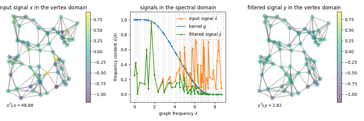
Filtering a signal

A graph signal is filtered by transforming it to the spectral domain (via the Fourier transform), performing a point-wise multiplication (motivated by the convolution theorem), and transforming it back to the vertex domain (via the inverse graph Fourier transform).

Note

In practice, filtering is implemented in the vertex domain to avoid the computationally expensive graph Fourier transform. To do so, filters are implemented as polynomials of the eigenvalues / Laplacian. Hence, filtering a signal reduces to its multiplications with sparse matrices (the graph Laplacian).

import numpy as np
from matplotlib import pyplot as plt
import pygsp as pg

G = pg.graphs.Sensor(seed=42)
G.compute_fourier_basis()

#g = pg.filters.Rectangular(G, band_max=0.2)
g = pg.filters.Expwin(G, band_max=0.5)

fig, axes = plt.subplots(1, 3, figsize=(12, 4))
fig.subplots_adjust(hspace=0.5)

x = np.random.default_rng(1).normal(size=G.N)
#x = np.random.default_rng(42).uniform(-1, 1, size=G.N)
x = 3 * x / np.linalg.norm(x)
y = g.filter(x)
x_hat = G.gft(x).squeeze()
y_hat = G.gft(y).squeeze()

limits = [x.min(), x.max()]

G.plot(x, limits=limits, ax=axes[0], title='input signal $x$ in the vertex domain')
axes[0].text(0, -0.1, '$x^T L x = {:.2f}$'.format(G.dirichlet_energy(x)))
axes[0].set_axis_off()

g.plot(ax=axes[1], alpha=1)
line_filt = axes[1].lines[-2]
line_in, = axes[1].plot(G.e, np.abs(x_hat), '.-')
line_out, = axes[1].plot(G.e, np.abs(y_hat), '.-')
#axes[1].set_xticks(range(0, 16, 4))
axes[1].set_xlabel(r'graph frequency $\lambda$')
axes[1].set_ylabel(r'frequency content $\hat{x}(\lambda)$')
axes[1].set_title(r'signals in the spectral domain')
axes[1].legend(['input signal $\hat{x}$'])
labels = [
    r'input signal $\hat{x}$',
    'kernel $g$',
    r'filtered signal $\hat{y}$',
]
axes[1].legend([line_in, line_filt, line_out], labels, loc='upper right')

G.plot(y, limits=limits, ax=axes[2], title='filtered signal $y$ in the vertex domain')
axes[2].text(0, -0.1, '$y^T L y = {:.2f}$'.format(G.dirichlet_energy(y)))
axes[2].set_axis_off()

fig.tight_layout()

Estimated memory usage: 9 MB