Graphs¶

The pygsp.graphs module implements the graph class hierarchy. A graph object is either constructed from an adjacency matrix, or by instantiating one of the built-in graph models.

Interface¶

The Graph base class allows to construct a graph object from any adjacency matrix and provides a common interface to that object. Derived classes then allows to instantiate various standard graph models.

Matrix operators¶

`Graph.W`
`Graph.L`
`Graph.U`	Fourier basis (eigenvectors of the Laplacian).
`Graph.D`	Differential operator (for gradient and divergence).

Checks¶

`Graph.check_weights`()	Check the characteristics of the weights matrix.
`Graph.is_connected`([recompute])	Check the strong connectivity of the graph (cached).
`Graph.is_directed`([recompute])	Check if the graph has directed edges (cached).

Attributes computation¶

`Graph.compute_laplacian`([lap_type])	Compute a graph Laplacian.
`Graph.estimate_lmax`([recompute])	Estimate the Laplacian’s largest eigenvalue (cached).
`Graph.compute_fourier_basis`([recompute])	Compute the Fourier basis of the graph (cached).
`Graph.compute_differential_operator`()	Compute the graph differential operator (cached).

Differential operators¶

`Graph.grad`(s)	Compute the gradient of a graph signal.
`Graph.div`(s)	Compute the divergence of a graph signal.

Localization¶

`Graph.modulate`(f, k)	Modulate the signal f to the frequency k.
`Graph.translate`(f, i)	Translate the signal f to the node i.

Transforms (frequency and vertex-frequency)¶

`Graph.gft`(s)	Compute the graph Fourier transform.
`Graph.igft`(s_hat)	Compute the inverse graph Fourier transform.
`Graph.gft_windowed`(g, f[, lowmemory])	Windowed graph Fourier transform.
`Graph.gft_windowed_gabor`(s, k)	Gabor windowed graph Fourier transform.
`Graph.gft_windowed_normalized`(g, f[, lowmemory])	Normalized windowed graph Fourier transform.

Plotting¶

`Graph.plot`(**kwargs)	Plot the graph.
`Graph.plot_signal`(signal, **kwargs)	Plot a signal on that graph.
`Graph.plot_spectrogram`(**kwargs)	Plot the graph’s spectrogram.

Others¶

`Graph.get_edge_list`()	Return an edge list, an alternative representation of the graph.
`Graph.set_coordinates`([kind])	Set node’s coordinates (their position when plotting).
`Graph.subgraph`(ind)	Create a subgraph given indices.
`Graph.extract_components`()	Split the graph into connected components.

Graph models¶

`Airfoil`(**kwargs)	Airfoil graph.
`BarabasiAlbert`([N, m0, m, seed])	Barabasi-Albert preferential attachment.
`Comet`([N, k])	Comet graph.
`Community`([N, Nc, min_comm, min_deg, …])	Community graph.
`DavidSensorNet`([N, seed])	Sensor network.
`ErdosRenyi`([N, p, directed, self_loops, …])	Erdos Renyi graph.
`FullConnected`([N])	Fully connected graph.
`Grid2d`([N1, N2])	2-dimensional grid graph.
`Logo`(**kwargs)	GSP logo.
`LowStretchTree`([k])	Low stretch tree.
`Minnesota`([connect])	Minnesota road network (from MatlabBGL).
`Path`([N])	Path graph.
`RandomRegular`([N, k, maxIter, seed])	Random k-regular graph.
`RandomRing`([N, seed])	Ring graph with randomly sampled nodes.
`Ring`([N, k])	K-regular ring graph.
`Sensor`([N, Nc, regular, n_try, distribute, …])	Random sensor graph.
`StochasticBlockModel`([N, k, z, M, p, q, …])	Stochastic Block Model (SBM).
`SwissRoll`([N, a, b, dim, thresh, s, noise, …])	Sampled Swiss roll manifold.
`Torus`([Nv, Mv])	Sampled torus manifold.

Nearest-neighbors graphs constructed from point clouds¶

`NNGraph`(Xin[, NNtype, use_flann, center, …])	Nearest-neighbor graph from given point cloud.
`Bunny`(**kwargs)	Stanford bunny (NN-graph).
`Cube`([radius, nb_pts, nb_dim, sampling, seed])	Hyper-cube (NN-graph).
`ImgPatches`(img[, patch_shape])	NN-graph between patches of an image.
`Grid2dImgPatches`(img[, aggregate])	Union of a patch graph with a 2D grid graph.
`Sphere`([radius, nb_pts, nb_dim, sampling, seed])	Spherical-shaped graph (NN-graph).
`TwoMoons`([moontype, dim, sigmag, N, sigmad, …])	Two Moons (NN-graph).

class pygsp.graphs.Graph(W, gtype='unknown', lap_type='combinatorial', coords=None, plotting={})[source]¶

Base graph class.

Provide a common interface (and implementation) to graph objects.
Can be instantiated to construct custom graphs from a weight matrix.
Initialize attributes for derived classes.

Parameters:

W : sparse matrix or ndarray

The weight matrix which encodes the graph.

gtype : string

Graph type, a free-form string to help us recognize the kind of graph we are dealing with (default is ‘unknown’).

lap_type : ‘combinatorial’, ‘normalized’

The type of Laplacian to be computed by compute_laplacian() (default is ‘combinatorial’).

coords : ndarray

Vertices coordinates (default is None).

plotting : dict

Plotting parameters.

Examples

>>> W = np.arange(4).reshape(2, 2)
>>> G = graphs.Graph(W)

Attributes

N	(int) the number of nodes / vertices in the graph.
Ne	(int) the number of edges / links in the graph, i.e. connections between nodes.
W	(sparse matrix) the weight matrix which contains the weights of the connections. It is represented as an N-by-N matrix of floats. \(W_{i,j} = 0\) means that there is no direct connection from i to j.
gtype	(string) the graph type is a short description of the graph object designed to help sorting the graphs.
L	(sparse matrix) the graph Laplacian, an N-by-N matrix computed from W.
lap_type	(‘normalized’, ‘combinatorial’) the kind of Laplacian that was computed by `compute_laplacian()`.
coords	(ndarray) vertices coordinates in 2D or 3D space. Used for plotting only. Default is None.
plotting	(dict) plotting parameters.

check_weights()[source]¶

Check the characteristics of the weights matrix.

Returns:

A dict of bools containing informations about the matrix

has_inf_val : bool

True if the matrix has infinite values else false

has_nan_value : bool

True if the matrix has a “not a number” value else false

is_not_square : bool

True if the matrix is not square else false

diag_is_not_zero : bool

True if the matrix diagonal has not only zeros else false

Examples

>>> W = np.arange(4).reshape(2, 2)
>>> G = graphs.Graph(W)
>>> cw = G.check_weights()
>>> cw == {'has_inf_val': False, 'has_nan_value': False,
...        'is_not_square': False, 'diag_is_not_zero': True}
True

compute_differential_operator()¶

Compute the graph differential operator (cached).

The differential operator is a matrix such that

\[L = D^T D,\]

where \(D\) is the differential operator and \(L\) is the graph Laplacian. It is used to compute the gradient and the divergence of a graph signal, see grad() and div().

The result is cached and accessible by the D property.

See also

compute_differential_operator

div: compute the divergence

Examples

>>> G = graphs.Logo()
>>> G.N, G.Ne
(1130, 3131)
>>> s = np.random.normal(size=G.N)
>>> s_grad = G.grad(s)
>>> s_div = G.div(s_grad)
>>> np.linalg.norm(s_div - G.L.dot(s)) < 1e-10
True

igft(s_hat)¶

Compute the inverse graph Fourier transform.

The inverse graph Fourier transform of a Fourier domain signal \(\hat{s}\) is defined as

\[s = U \hat{s},\]

where \(U\) is the Fourier basis U.

Parameters:

s_hat : ndarray

Graph signal in the Fourier domain.

Returns:

s : ndarray

Representation of s_hat in the vertex domain.

Examples

>>> G = graphs.Logo()
>>> G.compute_fourier_basis()
>>> s_hat = np.random.normal(size=(G.N, 5, 1))
>>> s = G.igft(s_hat)
>>> s_hat_star = G.gft(s)
>>> np.all((s_hat - s_hat_star) < 1e-10)
True

is_connected(recompute=False)[source]¶

Check the strong connectivity of the graph (cached).

It uses DFS travelling on graph to ensure that each node is visited. For undirected graphs, starting at any vertex and trying to access all others is enough. For directed graphs, one needs to check that a random vertex is accessible by all others and can access all others. Thus, we can transpose the adjacency matrix and compute again with the same starting point in both phases.

Parameters:

recompute: bool

Force to recompute the connectivity if already known.

Returns:

connected : bool

True if the graph is connected.

Examples

>>> from scipy import sparse
>>> W = sparse.rand(10, 10, 0.2)
>>> G = graphs.Graph(W=W)
>>> connected = G.is_connected()

is_directed(recompute=False)[source]¶

Check if the graph has directed edges (cached).

In this framework, we consider that a graph is directed if and only if its weight matrix is non symmetric.

Parameters:

recompute : bool

Force to recompute the directedness if already known.

Returns:

directed : bool

True if the graph is directed.

Notes

Can also be used to check if a matrix is symmetrical

Examples

>>> from scipy import sparse
>>> W = sparse.rand(10, 10, 0.2)
>>> G = graphs.Graph(W=W)
>>> directed = G.is_directed()

modulate(f, k)[source]¶

Modulate the signal f to the frequency k.

Parameters:

f : ndarray

Signal (column)

k : int

Index of frequencies

Returns:

fm : ndarray

Modulated signal

plot(**kwargs)[source]¶

Plot the graph.

See pygsp.plotting.plot_graph().

plot_signal(signal, **kwargs)[source]¶

Plot a signal on that graph.

See pygsp.plotting.plot_signal().

plot_spectrogram(**kwargs)[source]¶

Plot the graph’s spectrogram.

See pygsp.plotting.plot_spectrogram().

set_coordinates(kind='spring', **kwargs)[source]¶

Set node’s coordinates (their position when plotting).

Parameters:

kind : string or array-like

Kind of coordinates to generate. It controls the position of the nodes when plotting the graph. Can either pass an array of size Nx2 or Nx3 to set the coordinates manually or the name of a layout algorithm. Available algorithms: community2D, random2D, random3D, ring2D, line1D, spring. Default is ‘spring’.

kwargs : dict

Additional parameters to be passed to the Fruchterman-Reingold force-directed algorithm when kind is spring.

Examples

>>> G = graphs.ErdosRenyi()
>>> G.set_coordinates()
>>> G.plot()

subgraph(ind)[source]¶

Create a subgraph given indices.

Parameters:

ind : list

Nodes to keep

Returns:

sub_G : Graph

Subgraph

Examples

>>> W = np.arange(16).reshape(4, 4)
>>> G = graphs.Graph(W)
>>> ind = [1, 3]
>>> sub_G = G.subgraph(ind)

translate(f, i)¶

Translate the signal f to the node i.

Parameters:

f : ndarray

Signal

i : int

Indices of vertex

Returns:

ft : translate signal

A¶

Graph adjacency matrix (the binary version of W).

The adjacency matrix defines which edges exist on the graph. It is represented as an N-by-N matrix of booleans. \(A_{i,j}\) is True if \(W_{i,j} > 0\).

D¶

Differential operator (for gradient and divergence).

Is computed by compute_differential_operator().

U¶

Fourier basis (eigenvectors of the Laplacian).

Is computed by compute_fourier_basis().

d¶: The degree (the number of neighbors) of each node.

dw¶: The weighted degree (the sum of weighted edges) of each node.

e¶

Eigenvalues of the Laplacian (square of graph frequencies).

Is computed by compute_fourier_basis().

lmax¶

Largest eigenvalue of the graph Laplacian.

Can be exactly computed by compute_fourier_basis() or approximated by estimate_lmax().

mu¶

Coherence of the Fourier basis.

Is computed by compute_fourier_basis().

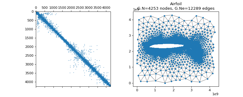
class pygsp.graphs.Airfoil(**kwargs)[source]¶

Airfoil graph.

Examples

>>> import matplotlib.pyplot as plt
>>> G = graphs.Airfoil()
>>> fig, axes = plt.subplots(1, 2)
>>> _ = axes[0].spy(G.W, markersize=0.5)
>>> G.plot(show_edges=True, ax=axes[1])

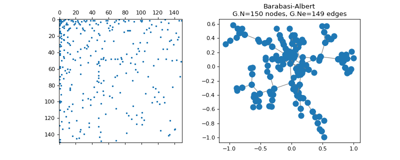
class pygsp.graphs.BarabasiAlbert(N=1000, m0=1, m=1, seed=None, **kwargs)[source]¶

Barabasi-Albert preferential attachment.

The Barabasi-Albert graph is constructed by connecting nodes in two steps. First, m0 nodes are created. Then, nodes are added one by one.

By lack of clarity, we take the liberty to create it as follows:

the m0 initial nodes are disconnected,

each node is connected to m of the older nodes with a probability distribution depending of the node-degrees of the other nodes, \(p_n(i) = \frac{1 + k_i}{\sum_j{1 + k_j}}\).

Parameters:

N : int

Number of nodes (default is 1000)

m0 : int

Number of initial nodes (default is 1)

m : int

Number of connections at each step (default is 1) m can never be larger than m0.

seed : int

Seed for the random number generator (for reproducible graphs).

Examples

>>> import matplotlib.pyplot as plt
>>> G = graphs.BarabasiAlbert(N=150, seed=42)
>>> G.set_coordinates(kind='spring', seed=42)
>>> fig, axes = plt.subplots(1, 2)
>>> _ = axes[0].spy(G.W, markersize=2)
>>> G.plot(ax=axes[1])

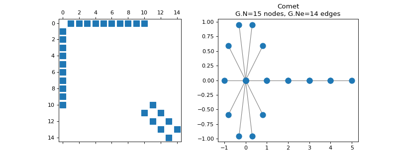
class pygsp.graphs.Comet(N=32, k=12, **kwargs)[source]¶

Comet graph.

The comet graph is a path graph with a star of degree k at its end.

Parameters:

N : int

Number of nodes.

k : int

Degree of center vertex.

Examples

>>> import matplotlib.pyplot as plt
>>> G = graphs.Comet(15, 10)
>>> fig, axes = plt.subplots(1, 2)
>>> _ = axes[0].spy(G.W)
>>> G.plot(ax=axes[1])

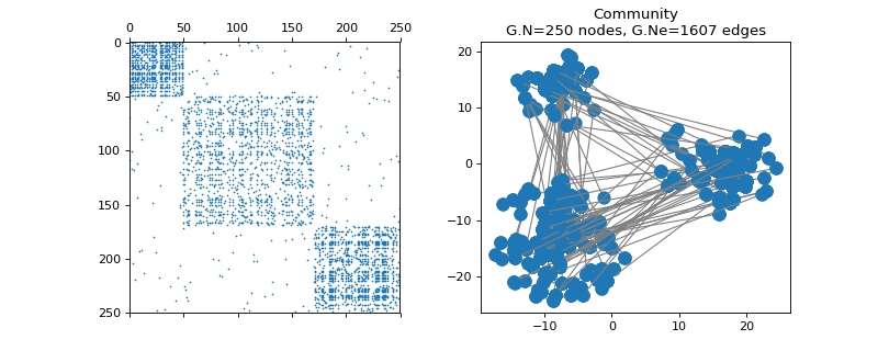
class pygsp.graphs.Community(N=256, Nc=None, min_comm=None, min_deg=0, comm_sizes=None, size_ratio=1, world_density=None, comm_density=None, k_neigh=None, epsilon=None, seed=None, **kwargs)[source]¶

Community graph.

Parameters:

N : int

Number of nodes (default = 256).

Nc : int (optional)

Number of communities (default = \(\lfloor \sqrt{N}/2 \rceil\)).

min_comm : int (optional)

Minimum size of the communities (default = \(\lfloor N/Nc/3 \rceil\)).

min_deg : int (optional)

NOT IMPLEMENTED. Minimum degree of each node (default = 0).

comm_sizes : int (optional)

Size of the communities (default = random).

size_ratio : float (optional)

Ratio between the radius of world and the radius of communities (default = 1).

world_density : float (optional)

Probability of a random edge between two different communities (default = 1/N).

comm_density : float (optional)

Probability of a random edge inside any community (default = None, which implies k_neigh or epsilon will be used to determine intra-edges).

k_neigh : int (optional)

Number of intra-community connections. Not used if comm_density is defined (default = None, which implies comm_density or epsilon will be used to determine intra-edges).

epsilon : float (optional)

Largest distance at which two nodes sharing a community are connected. Not used if k_neigh or comm_density is defined (default = \(\sqrt{2\sqrt{N}}/2\)).

seed : int

Seed for the random number generator (for reproducible graphs).

Examples

>>> import matplotlib.pyplot as plt
>>> G = graphs.Community(N=250, Nc=3, comm_sizes=[50, 120, 80], seed=42)
>>> fig, axes = plt.subplots(1, 2)
>>> _ = axes[0].spy(G.W, markersize=0.5)
>>> G.plot(ax=axes[1])

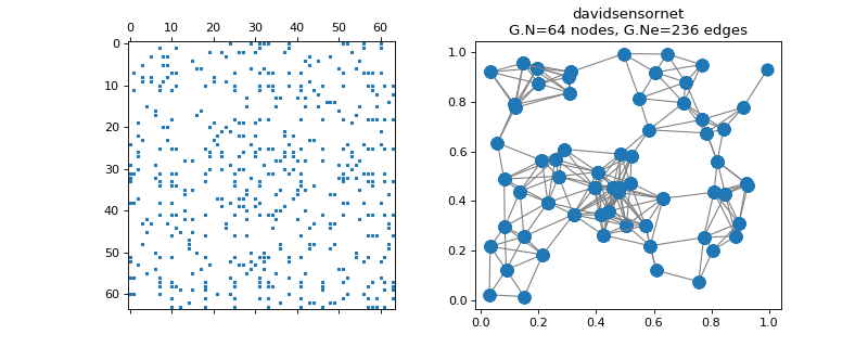
class pygsp.graphs.DavidSensorNet(N=64, seed=None, **kwargs)[source]¶

Sensor network.

Parameters:

N : int

Number of vertices (default = 64). Values of 64 and 500 yield pre-computed and saved graphs. Other values yield randomly generated graphs.

seed : int

Seed for the random number generator (for reproducible graphs).

Examples

>>> import matplotlib.pyplot as plt
>>> G = graphs.DavidSensorNet()
>>> fig, axes = plt.subplots(1, 2)
>>> _ = axes[0].spy(G.W, markersize=2)
>>> G.plot(ax=axes[1])

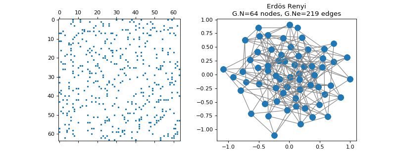
class pygsp.graphs.ErdosRenyi(N=100, p=0.1, directed=False, self_loops=False, connected=False, max_iter=10, seed=None, **kwargs)[source]¶

Erdos Renyi graph.

The Erdos Renyi graph is constructed by randomly connecting nodes. Each edge is included in the graph with probability p, independently from any other edge. All edge weights are equal to 1.

Parameters:

N : int

Number of nodes (default is 100).

p : float

Probability to connect a node with another one.

directed : bool

Allow directed edges if True (default is False).

self_loops : bool

Allow self loops if True (default is False).

connected : bool

Force the graph to be connected (default is False).

max_iter : int

Maximum number of trials to get a connected graph (default is 10).

seed : int

Seed for the random number generator (for reproducible graphs).

Examples

>>> import matplotlib.pyplot as plt
>>> G = graphs.ErdosRenyi(N=64, seed=42)
>>> G.set_coordinates(kind='spring', seed=42)
>>> fig, axes = plt.subplots(1, 2)
>>> _ = axes[0].spy(G.W, markersize=2)
>>> G.plot(ax=axes[1])

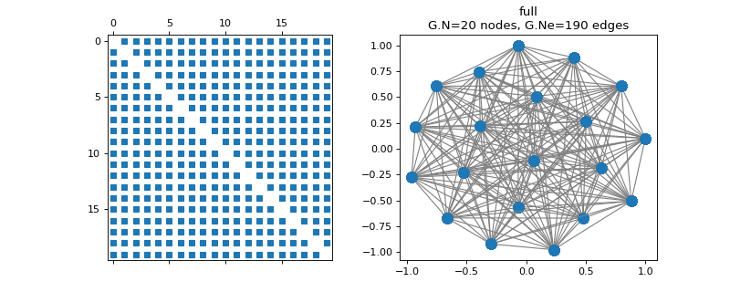
class pygsp.graphs.FullConnected(N=10, **kwargs)[source]¶

Fully connected graph.

All weights are set to 1. There is no self-connections.

Parameters:

N : int

Number of vertices (default = 10)

Examples

>>> import matplotlib.pyplot as plt
>>> G = graphs.FullConnected(N=20)
>>> G.set_coordinates(kind='spring', seed=42)
>>> fig, axes = plt.subplots(1, 2)
>>> _ = axes[0].spy(G.W, markersize=5)
>>> G.plot(ax=axes[1])

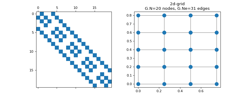
class pygsp.graphs.Grid2d(N1=16, N2=None, **kwargs)[source]¶

2-dimensional grid graph.

Parameters:

N1 : int

Number of vertices along the first dimension.

N2 : int

Number of vertices along the second dimension (default N1).

Examples

>>> import matplotlib.pyplot as plt
>>> G = graphs.Grid2d(N1=5, N2=4)
>>> fig, axes = plt.subplots(1, 2)
>>> _ = axes[0].spy(G.W)
>>> G.plot(ax=axes[1])

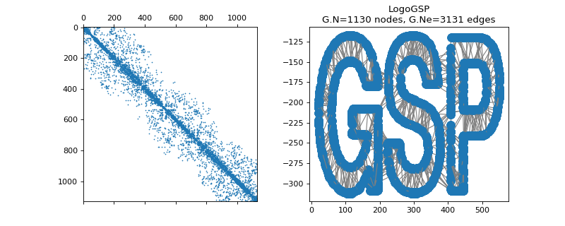
class pygsp.graphs.Logo(**kwargs)[source]¶

GSP logo.

Examples

>>> import matplotlib.pyplot as plt
>>> G = graphs.Logo()
>>> fig, axes = plt.subplots(1, 2)
>>> _ = axes[0].spy(G.W, markersize=0.5)
>>> G.plot(ax=axes[1])

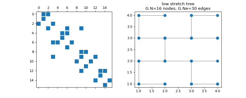
class pygsp.graphs.LowStretchTree(k=6, **kwargs)[source]¶

Low stretch tree.

Build the root of a low stretch tree on a grid of points. There are \(2k\) points on each side of the grid, and therefore \(2^{2k}\) vertices in total. The edge weights are all equal to 1.

Parameters:

k : int

\(2^k\) points on each side of the grid of vertices.

Examples

>>> import matplotlib.pyplot as plt
>>> G = graphs.LowStretchTree(k=2)
>>> fig, axes = plt.subplots(1, 2)
>>> _ = axes[0].spy(G.W)
>>> G.plot(ax=axes[1])

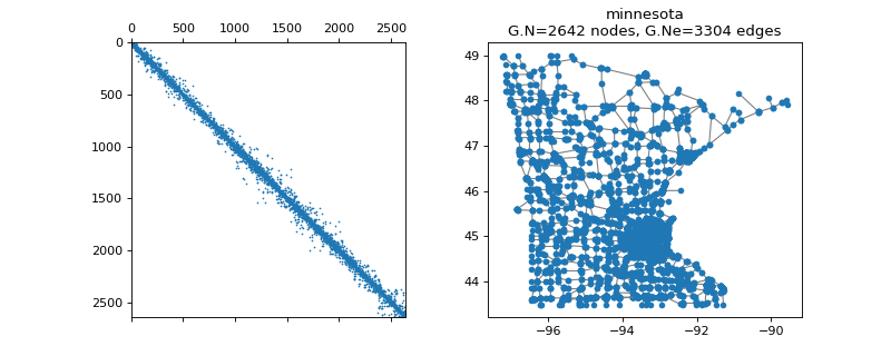
class pygsp.graphs.Minnesota(connect=True, **kwargs)[source]¶

Minnesota road network (from MatlabBGL).

Parameters:

connect : bool

If True, the adjacency matrix is adjusted so that all edge weights are equal to 1, and the graph is connected. Set to False to get the original disconnected graph.

References

See [Gle].

Examples

>>> import matplotlib.pyplot as plt
>>> G = graphs.Minnesota()
>>> fig, axes = plt.subplots(1, 2)
>>> _ = axes[0].spy(G.W, markersize=0.5)
>>> G.plot(ax=axes[1])

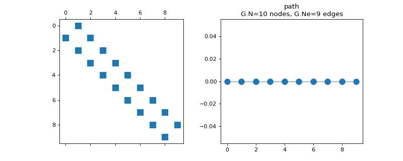
class pygsp.graphs.Path(N=16, **kwargs)[source]¶

Path graph.

Parameters:

N : int

Number of vertices.

References

See [Str99] for more informations.

Examples

>>> import matplotlib.pyplot as plt
>>> G = graphs.Path(N=10)
>>> fig, axes = plt.subplots(1, 2)
>>> _ = axes[0].spy(G.W)
>>> G.plot(ax=axes[1])

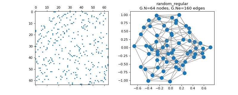
class pygsp.graphs.RandomRegular(N=64, k=6, maxIter=10, seed=None, **kwargs)[source]¶

Random k-regular graph.

The random regular graph has the property that every node is connected to k other nodes. That graph is simple (without loops or double edges), k-regular (each vertex is adjacent to k nodes), and undirected.

Parameters:

N : int

Number of nodes (default is 64)

k : int

Number of connections, or degree, of each node (default is 6)

maxIter : int

Maximum number of iterations (default is 10)

seed : int

Seed for the random number generator (for reproducible graphs).

Notes

The pairing model algorithm works as follows. First create n*d half edges. Then repeat as long as possible: pick a pair of half edges and if it’s legal (doesn’t create a loop nor a double edge) add it to the graph.

References

See [KV03]. This code has been adapted from matlab to python.

Examples

>>> import matplotlib.pyplot as plt
>>> G = graphs.RandomRegular(N=64, k=5, seed=42)
>>> G.set_coordinates(kind='spring', seed=42)
>>> fig, axes = plt.subplots(1, 2)
>>> _ = axes[0].spy(G.W, markersize=2)
>>> G.plot(ax=axes[1])

is_regular()[source]¶: Troubleshoot a given regular graph.

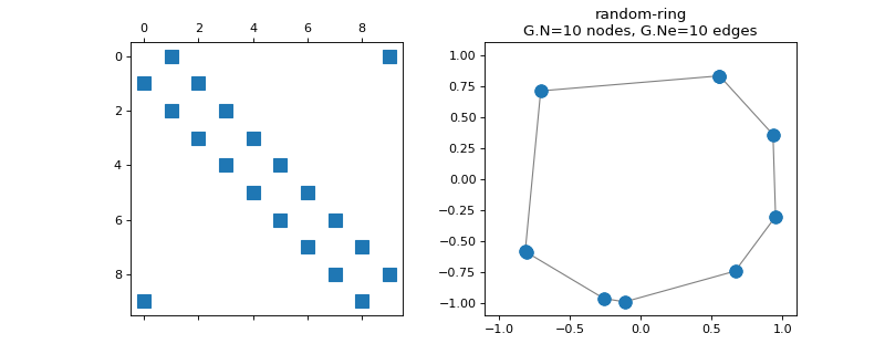
class pygsp.graphs.RandomRing(N=64, seed=None, **kwargs)[source]¶

Ring graph with randomly sampled nodes.

Parameters:

N : int

Number of vertices.

seed : int

Seed for the random number generator (for reproducible graphs).

Examples

>>> import matplotlib.pyplot as plt
>>> G = graphs.RandomRing(N=10, seed=42)
>>> fig, axes = plt.subplots(1, 2)
>>> _ = axes[0].spy(G.W)
>>> G.plot(ax=axes[1])
>>> _ = axes[1].set_xlim(-1.1, 1.1)
>>> _ = axes[1].set_ylim(-1.1, 1.1)

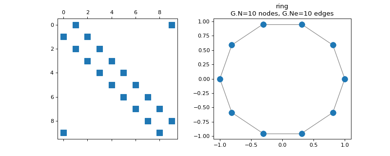
class pygsp.graphs.Ring(N=64, k=1, **kwargs)[source]¶

K-regular ring graph.

Parameters:

N : int

Number of vertices.

k : int

Number of neighbors in each direction.

Examples

>>> import matplotlib.pyplot as plt
>>> G = graphs.Ring(N=10)
>>> fig, axes = plt.subplots(1, 2)
>>> _ = axes[0].spy(G.W)
>>> G.plot(ax=axes[1])

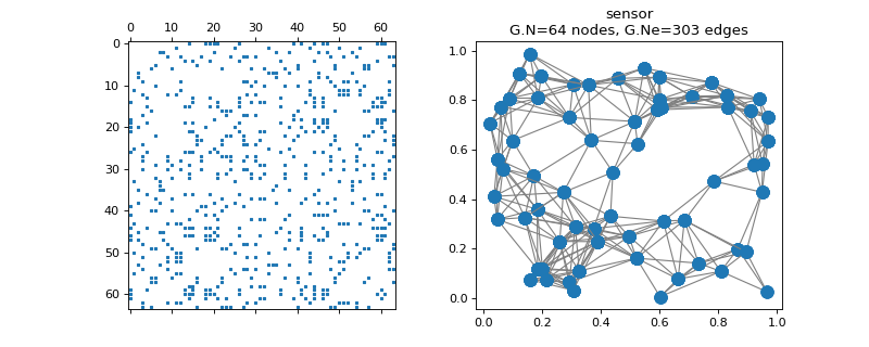
class pygsp.graphs.Sensor(N=64, Nc=2, regular=False, n_try=50, distribute=False, connected=True, seed=None, **kwargs)[source]¶

Random sensor graph.

Parameters:

N : int

Number of nodes (default = 64)

Nc : int

Minimum number of connections (default = 2)

regular : bool

Flag to fix the number of connections to nc (default = False)

n_try : int

Number of attempt to create the graph (default = 50)

distribute : bool

To distribute the points more evenly (default = False)

connected : bool

To force the graph to be connected (default = True)

seed : int

Seed for the random number generator (for reproducible graphs).

Examples

>>> import matplotlib.pyplot as plt
>>> G = graphs.Sensor(N=64, seed=42)
>>> fig, axes = plt.subplots(1, 2)
>>> _ = axes[0].spy(G.W, markersize=2)
>>> G.plot(ax=axes[1])

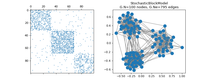
class pygsp.graphs.StochasticBlockModel(N=1024, k=5, z=None, M=None, p=0.7, q=None, directed=False, self_loops=False, connected=False, max_iter=10, seed=None, **kwargs)[source]¶

Stochastic Block Model (SBM).

The Stochastic Block Model graph is constructed by connecting nodes with a probability which depends on the cluster of the two nodes. One can define the clustering association of each node, denoted by vector z, but also the probability matrix M. All edge weights are equal to 1. By default, Mii > Mjk and nodes are uniformly clusterized.

Parameters:

N : int

Number of nodes (default is 1024).

k : float

Number of classes (default is 5).

z : array_like

the vector of length N containing the association between nodes and classes (default is random uniform).

M : array_like

the k by k matrix containing the probability of connecting nodes based on their class belonging (default using p and q).

p : float or array_like

the diagonal value(s) for the matrix M. If scalar they all have the same value. Otherwise expect a length k vector (default is p = 0.7).

q : float or array_like

the off-diagonal value(s) for the matrix M. If scalar they all have the same value. Otherwise expect a k x k matrix, diagonal will be discarded (default is q = 0.3/k).

directed : bool

Allow directed edges if True (default is False).

self_loops : bool

Allow self loops if True (default is False).

connected : bool

Force the graph to be connected (default is False).

max_iter : int

Maximum number of trials to get a connected graph (default is 10).

seed : int

Seed for the random number generator (for reproducible graphs).

Examples

>>> import matplotlib.pyplot as plt
>>> G = graphs.StochasticBlockModel(
...     100, k=3, p=[0.4, 0.6, 0.3], q=0.02, seed=42)
>>> G.set_coordinates(kind='spring', seed=42)
>>> fig, axes = plt.subplots(1, 2)
>>> _ = axes[0].spy(G.W, markersize=0.8)
>>> G.plot(ax=axes[1])

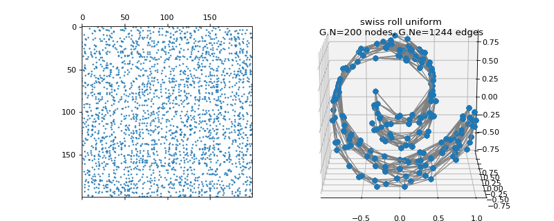
class pygsp.graphs.SwissRoll(N=400, a=1, b=4, dim=3, thresh=1e-06, s=None, noise=False, srtype='uniform', seed=None, **kwargs)[source]¶

Sampled Swiss roll manifold.

Parameters:

N : int

Number of vertices (default = 400)

a : int

(default = 1)

b : int

(default = 4)

dim : int

(default = 3)

thresh : float

(default = 1e-6)

s : float

sigma (default = sqrt(2./N))

noise : bool

Wether to add noise or not (default = False)

srtype : str

Swiss roll Type, possible arguments are ‘uniform’ or ‘classic’ (default = ‘uniform’)

seed : int

Seed for the random number generator (for reproducible graphs).

Examples

>>> import matplotlib.pyplot as plt
>>> G = graphs.SwissRoll(N=200, seed=42)
>>> fig = plt.figure()
>>> ax1 = fig.add_subplot(121)
>>> ax2 = fig.add_subplot(122, projection='3d')
>>> _ = ax1.spy(G.W, markersize=1)
>>> G.plot(ax=ax2)

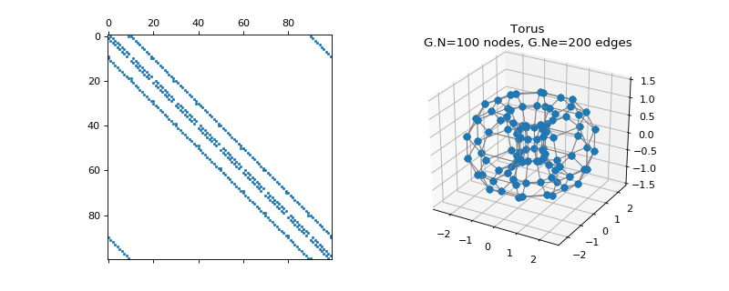
class pygsp.graphs.Torus(Nv=16, Mv=None, **kwargs)[source]¶

Sampled torus manifold.

Parameters:

Nv : int

Number of vertices along the first dimension (default is 16)

Mv : int

Number of vertices along the second dimension (default is Nv)

References

See [Str99] for more informations.

Examples

>>> import matplotlib.pyplot as plt
>>> G = graphs.Torus(10)
>>> fig = plt.figure()
>>> ax1 = fig.add_subplot(121)
>>> ax2 = fig.add_subplot(122, projection='3d')
>>> _ = ax1.spy(G.W, markersize=1.5)
>>> G.plot(ax=ax2)
>>> _ = ax2.set_zlim(-1.5, 1.5)

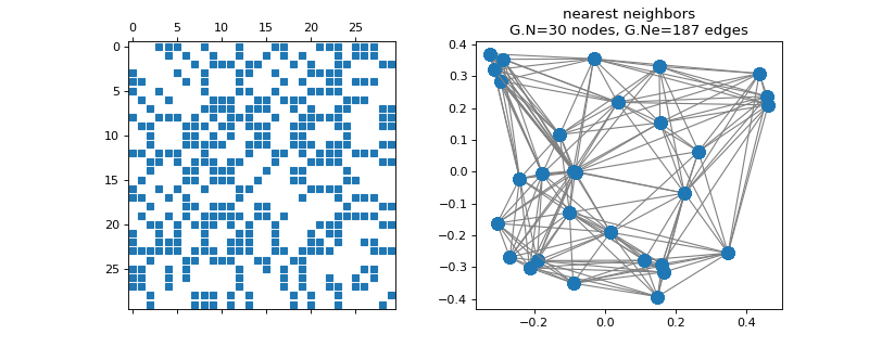
class pygsp.graphs.NNGraph(Xin, NNtype='knn', use_flann=False, center=True, rescale=True, k=10, sigma=0.1, epsilon=0.01, gtype=None, plotting={}, symmetrize_type='average', dist_type='euclidean', order=0, **kwargs)[source]¶

Nearest-neighbor graph from given point cloud.

Parameters:

Xin : ndarray

Input points, Should be an N-by-d matrix, where N is the number of nodes in the graph and d is the dimension of the feature space.

NNtype : string, optional

Type of nearest neighbor graph to create. The options are ‘knn’ for k-Nearest Neighbors or ‘radius’ for epsilon-Nearest Neighbors (default is ‘knn’).

use_flann : bool, optional

Use Fast Library for Approximate Nearest Neighbors (FLANN) or not. (default is False)

center : bool, optional

Center the data so that it has zero mean (default is True)

rescale : bool, optional

Rescale the data so that it lies in a l2-sphere (default is True)

k : int, optional

Number of neighbors for knn (default is 10)

sigma : float, optional

Width parameter of the similarity kernel (default is 0.1)

epsilon : float, optional

Radius for the epsilon-neighborhood search (default is 0.01)

gtype : string, optional

The type of graph (default is ‘nearest neighbors’)

plotting : dict, optional

Dictionary of plotting parameters. See pygsp.plotting. (default is {})

symmetrize_type : string, optional

Type of symmetrization to use for the adjacency matrix. See pygsp.utils.symmetrization() for the options. (default is ‘average’)

dist_type : string, optional

Type of distance to compute. See pyflann.index.set_distance_type() for possible options. (default is ‘euclidean’)

order : float, optional

Only used if dist_type is ‘minkowski’; represents the order of the Minkowski distance. (default is 0)

Examples

>>> import matplotlib.pyplot as plt
>>> X = np.random.RandomState(42).uniform(size=(30, 2))
>>> G = graphs.NNGraph(X)
>>> fig, axes = plt.subplots(1, 2)
>>> _ = axes[0].spy(G.W, markersize=5)
>>> G.plot(ax=axes[1])

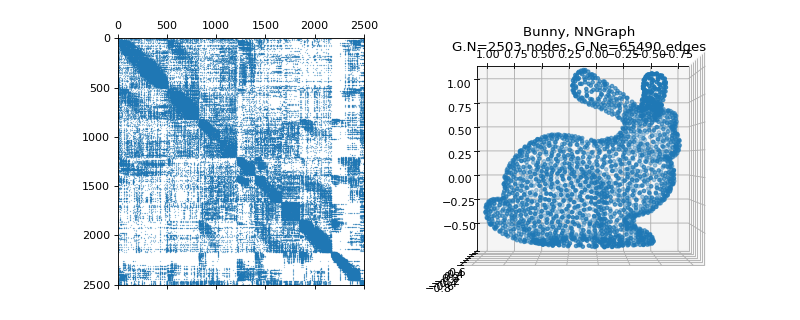
class pygsp.graphs.Bunny(**kwargs)[source]¶

Stanford bunny (NN-graph).

References

See [TL94].

Examples

>>> import matplotlib.pyplot as plt
>>> G = graphs.Bunny()
>>> fig = plt.figure()
>>> ax1 = fig.add_subplot(121)
>>> ax2 = fig.add_subplot(122, projection='3d')
>>> _ = ax1.spy(G.W, markersize=0.1)
>>> G.plot(ax=ax2)

class pygsp.graphs.Cube(radius=1, nb_pts=300, nb_dim=3, sampling='random', seed=None, **kwargs)[source]¶

Hyper-cube (NN-graph).

Parameters:

radius : float

Edge lenght (default = 1)

nb_pts : int

Number of vertices (default = 300)

nb_dim : int

Dimension (default = 3)

sampling : string

Variance of the distance kernel (default = ‘random’) (Can now only be ‘random’)

seed : int

Seed for the random number generator (for reproducible graphs).

Examples

>>> import matplotlib.pyplot as plt
>>> G = graphs.Cube(seed=42)
>>> fig = plt.figure()
>>> ax1 = fig.add_subplot(121)
>>> ax2 = fig.add_subplot(122, projection='3d')
>>> _ = ax1.spy(G.W, markersize=0.5)
>>> G.plot(ax=ax2)

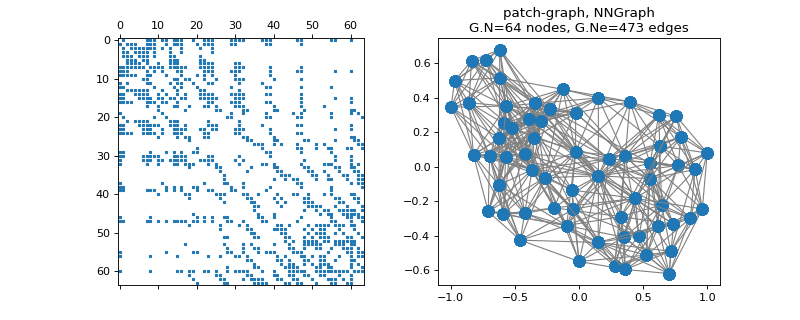
class pygsp.graphs.ImgPatches(img, patch_shape=(3, 3), **kwargs)[source]¶

NN-graph between patches of an image.

Extract a feature vector in the form of a patch for every pixel of an image, then construct a nearest-neighbor graph between these feature vectors. The feature matrix, i.e. the patches, can be found in Xin.

Parameters:

img : array

Input image.

patch_shape : tuple, optional

Dimensions of the patch window. Syntax: (height, width), or (height,), in which case width = height.

kwargs : dict

Parameters passed to NNGraph.

Notes

The feature vector of a pixel i will consist of the stacking of the intensity values of all pixels in the patch centered at i, for all color channels. So, if the input image has d color channels, the dimension of the feature vector of each pixel is (patch_shape[0] * patch_shape[1] * d).

Examples

>>> import matplotlib.pyplot as plt
>>> from skimage import data, img_as_float
>>> img = img_as_float(data.camera()[::64, ::64])
>>> G = graphs.ImgPatches(img, patch_shape=(3, 3))
>>> print('{} nodes ({} x {} pixels)'.format(G.Xin.shape[0], *img.shape))
64 nodes (8 x 8 pixels)
>>> print('{} features per node'.format(G.Xin.shape[1]))
9 features per node
>>> G.set_coordinates(kind='spring', seed=42)
>>> fig, axes = plt.subplots(1, 2)
>>> _ = axes[0].spy(G.W, markersize=2)
>>> G.plot(ax=axes[1])

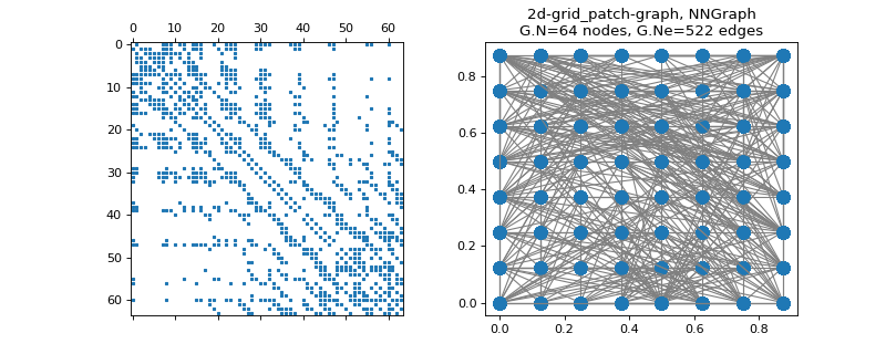
class pygsp.graphs.Grid2dImgPatches(img, aggregate=<function Grid2dImgPatches.<lambda>>, **kwargs)[source]¶

Union of a patch graph with a 2D grid graph.

Parameters:

img : array

Input image.

aggregate: callable, optional

Function to aggregate the weights Wp of the patch graph and the Wg of the grid graph. Default is lambda Wp, Wg: Wp + Wg.

kwargs : dict

Parameters passed to ImgPatches.

Examples

>>> import matplotlib.pyplot as plt
>>> from skimage import data, img_as_float
>>> img = img_as_float(data.camera()[::64, ::64])
>>> G = graphs.Grid2dImgPatches(img)
>>> fig, axes = plt.subplots(1, 2)
>>> _ = axes[0].spy(G.W, markersize=2)
>>> G.plot(ax=axes[1])

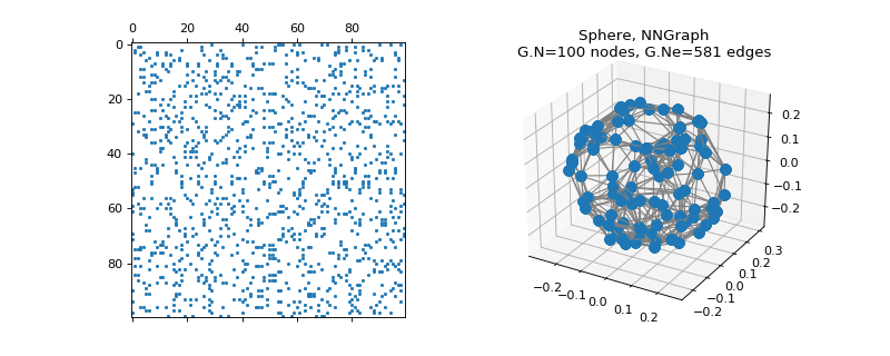
class pygsp.graphs.Sphere(radius=1, nb_pts=300, nb_dim=3, sampling='random', seed=None, **kwargs)[source]¶

Spherical-shaped graph (NN-graph).

Parameters:

radius : flaot

Radius of the sphere (default = 1)

nb_pts : int

Number of vertices (default = 300)

nb_dim : int

Dimension (default = 3)

sampling : sting

Variance of the distance kernel (default = ‘random’) (Can now only be ‘random’)

seed : int

Seed for the random number generator (for reproducible graphs).

Examples

>>> import matplotlib.pyplot as plt
>>> G = graphs.Sphere(nb_pts=100, seed=42)
>>> fig = plt.figure()
>>> ax1 = fig.add_subplot(121)
>>> ax2 = fig.add_subplot(122, projection='3d')
>>> _ = ax1.spy(G.W, markersize=1.5)
>>> G.plot(ax=ax2)

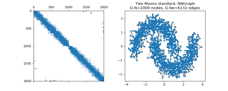
class pygsp.graphs.TwoMoons(moontype='standard', dim=2, sigmag=0.05, N=400, sigmad=0.07, d=0.5, seed=None, **kwargs)[source]¶

Two Moons (NN-graph).

Parameters:

moontype : ‘standard’ or ‘synthesized’

You have the freedom to chose if you want to create a standard two_moons graph or a synthesized one (default is ‘standard’). ‘standard’ : Create a two_moons graph from a based graph. ‘synthesized’ : Create a synthesized two_moon

sigmag : float

Variance of the distance kernel (default = 0.05)

dim : int

The dimensionality of the points (default = 2). Only valid for moontype == ‘standard’.

N : int

Number of vertices (default = 2000) Only valid for moontype == ‘synthesized’.

sigmad : float

Variance of the data (do not set it too high or you won’t see anything) (default = 0.05) Only valid for moontype == ‘synthesized’.

d : float

Distance of the two moons (default = 0.5) Only valid for moontype == ‘synthesized’.

seed : int

Seed for the random number generator (for reproducible graphs).

Examples

>>> import matplotlib.pyplot as plt
>>> G = graphs.TwoMoons()
>>> fig, axes = plt.subplots(1, 2)
>>> _ = axes[0].spy(G.W, markersize=0.5)
>>> G.plot(show_edges=True, ax=axes[1])