Filters¶

The pygsp.filters module implements methods used for filtering and defines commonly used filters that can be applied to pygsp.graphs. A filter is associated to a graph and is defined with one or several functions. We define by filter bank a list of filters, usually centered around different frequencies, applied to a single graph.

Interface¶

The Filter base class implements a common interface to all filters:

`Filter.evaluate`(x)	Evaluate the kernels at given frequencies.
`Filter.filter`(s[, method, order])	Filter signals (analysis or synthesis).
`Filter.analyze`(s[, method, order])	Convenience alias to `filter()`.
`Filter.synthesize`(s[, method, order])	Convenience wrapper around `filter()`.
`Filter.compute_frame`(**kwargs)	Compute the associated frame.
`Filter.estimate_frame_bounds`([min, max, N, …])	Estimate lower and upper frame bounds.
`Filter.plot`(**kwargs)	Plot the filter bank’s frequency response.
`Filter.localize`(i, **kwargs)	Localize the kernels at a node (to visualize them).

Filters¶

Then, derived classes implement various common graph filters.

Filter banks of N filters

`Abspline`(G[, Nf, lpfactor, scales])	Design an A B cubic spline wavelet filter bank.
`Gabor`(G, k)	Design a Gabor filter bank.
`HalfCosine`(G[, Nf])	Design an half cosine filter bank (tight frame).
`Itersine`(G[, Nf, overlap])	Design an itersine filter bank (tight frame).
`MexicanHat`(G[, Nf, lpfactor, scales, normalize])	Design a filter bank of Mexican hat wavelets.
`Meyer`(G[, Nf, scales])	Design a filter bank of Meyer wavelets (tight frame).
`SimpleTight`(G[, Nf, scales])	Design a simple tight frame filter bank (tight frame).

Filter banks of 2 filters: a low pass and a high pass

`Regular`(G[, d])	Design 2 filters with the regular construction (tight frame).
`Held`(G[, a])	Design 2 filters with the Held construction (tight frame).
`Simoncelli`(G[, a])	Design 2 filters with the Simoncelli construction (tight frame).
`Papadakis`(G[, a])	Design 2 filters with the Papadakis construction (tight frame).

Low pass filters

`Heat`(G[, tau, normalize])	Design a filter bank of heat kernels.
`Expwin`(G[, bmax, a])	Design an exponential window filter.

Approximations¶

Moreover, two approximation methods are provided for fast filtering. The computational complexity of filtering with those approximations is linear with the number of edges. The complexity of the exact solution, which is to use the Fourier basis, is quadratic with the number of nodes (without taking into account the cost of the necessary eigendecomposition of the graph Laplacian).

Chebyshev polynomials

`compute_cheby_coeff`(f[, m, N])	Compute Chebyshev coefficients for a Filterbank.
`compute_jackson_cheby_coeff`(filter_bounds, …)	To compute the m+1 coefficients of the polynomial approximation of an ideal band-pass between a and b, between a range of values defined by lambda_min and lambda_max.
`cheby_op`(G, c, signal, **kwargs)	Chebyshev polynomial of graph Laplacian applied to vector.
`cheby_rect`(G, bounds, signal, **kwargs)	Fast filtering using Chebyshev polynomial for a perfect rectangle filter.

Lanczos algorithm

`lanczos`(A, order, x)	TODO short description
`lanczos_op`(f, s[, order])	Perform the lanczos approximation of the signal s.

class pygsp.filters.Filter(G, kernels)[source]¶

The base Filter class.

Provide a common interface (and implementation) to filter objects.
Can be instantiated to construct custom filters from functions.
Initialize attributes for derived classes.

Parameters:

G : graph

The graph to which the filter bank is tailored.

kernels : function or list of functions

A (list of) function(s) defining the filter bank in the Fourier domain. One function per filter.

Examples

>>>
>>> G = graphs.Logo()
>>> my_filter = filters.Filter(G, lambda x: x / (1. + x))
>>>
>>> # Signal: Kronecker delta.
>>> signal = np.zeros(G.N)
>>> signal[42] = 1
>>>
>>> filtered_signal = my_filter.filter(signal)

Attributes

G	(Graph) The graph to which the filter bank was tailored. It is a reference to the graph passed when instantiating the class.
kernels	(function or list of functions) A (list of) function defining the filter bank. One function per filter. Either passed by the user when instantiating the base class, either constructed by the derived classes.
Nf	(int) Number of filters in the filter bank.

analyze(s, method='chebyshev', order=30)[source]¶: Convenience alias to filter().

can_dual()[source]¶: Creates a dual graph form a given graph

compute_frame(**kwargs)[source]¶

Compute the associated frame.

The size of the returned matrix operator \(D\) is N x MN, where M is the number of filters and N the number of nodes. Multiplying this matrix with a set of signals is equivalent to analyzing them with the associated filterbank. Though computing this matrix is a rather inefficient way of doing it.

The frame is defined as follows:

\[g_i(L) = U g_i(\Lambda) U^*,\]

where \(g\) is the filter kernel, \(L\) is the graph Laplacian, \(\Lambda\) is a diagonal matrix of the Laplacian’s eigenvalues, and \(U\) is the Fourier basis, i.e. its columns are the eigenvectors of the Laplacian.

Parameters:

kwargs: dict

Parameters to be passed to the analyze() method.

Returns:

frame : ndarray

Matrix of size N x MN.

See also

filter: more efficient way to filter signals

Examples

Filtering signals as a matrix multiplication.

>>> G = graphs.Sensor(N=1000, seed=42)
>>> G.estimate_lmax()
>>> f = filters.MexicanHat(G, Nf=6)
>>> s = np.random.uniform(size=G.N)
>>>
>>> frame = f.compute_frame()
>>> frame.shape
(1000, 1000, 6)
>>> frame = frame.reshape(G.N, -1).T
>>> s1 = np.dot(frame, s)
>>> s1 = s1.reshape(G.N, -1)
>>>
>>> s2 = f.filter(s)
>>> np.all((s1 - s2) < 1e-10)
True

estimate_frame_bounds(min=0, max=None, N=1000, use_eigenvalues=False)[source]¶

Estimate lower and upper frame bounds.

The frame bounds are estimated using the vector np.linspace(min, max, N) with min=0 and max=G.lmax by default. The eigenvalues G.e can be used instead if you set use_eigenvalues to True.

Parameters:

min : float

The lowest value the filter bank is evaluated at. By default filtering is bounded by the eigenvalues of G, i.e. min = 0.

max : float

The largest value the filter bank is evaluated at. By default filtering is bounded by the eigenvalues of G, i.e. max = G.lmax.

N : int

Number of points where the filter bank is evaluated. Default is 1000.

use_eigenvalues : bool

Set to True to use the Laplacian eigenvalues instead.

Returns:

A : float

Lower frame bound of the filter bank.

B : float

Upper frame bound of the filter bank.

Examples

>>> G = graphs.Logo()
>>> G.compute_fourier_basis()
>>> f = filters.MexicanHat(G)

Bad estimation:

>>> A, B = f.estimate_frame_bounds(min=1, max=20, N=100)
>>> print('A={:.3f}, B={:.3f}'.format(A, B))
A=0.125, B=0.270

Better estimation:

>>> A, B = f.estimate_frame_bounds()
>>> print('A={:.3f}, B={:.3f}'.format(A, B))
A=0.177, B=0.270

Best estimation:

>>> G.compute_fourier_basis()
>>> A, B = f.estimate_frame_bounds(use_eigenvalues=True)
>>> print('A={:.3f}, B={:.3f}'.format(A, B))
A=0.177, B=0.270

The Itersine filter bank defines a tight frame:

>>> f = filters.Itersine(G)
>>> A, B = f.estimate_frame_bounds(use_eigenvalues=True)
>>> print('A={:.3f}, B={:.3f}'.format(A, B))
A=1.000, B=1.000

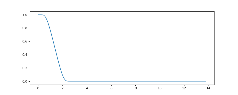
evaluate(x)[source]¶

Evaluate the kernels at given frequencies.

Parameters:

x : ndarray

Graph frequencies at which to evaluate the filter.

Returns:

y : ndarray

Frequency response of the filters. Shape (G.Nf, len(x)).

Examples

Frequency response of a low-pass filter:

>>> import matplotlib.pyplot as plt
>>> G = graphs.Logo()
>>> G.compute_fourier_basis()
>>> f = filters.Expwin(G)
>>> G.compute_fourier_basis()
>>> y = f.evaluate(G.e)
>>> plt.plot(G.e, y[0])  
[<matplotlib.lines.Line2D object at ...>]

filter(s, method='chebyshev', order=30)[source]¶

Filter signals (analysis or synthesis).

A signal is defined as a rank-3 tensor of shape (N_NODES, N_SIGNALS, N_FEATURES), where N_NODES is the number of nodes in the graph, N_SIGNALS is the number of independent signals, and N_FEATURES is the number of features which compose a graph signal, or the dimensionality of a graph signal. For example if you filter a signal with a filter bank of 8 filters, you’re extracting 8 features and decomposing your signal into 8 parts. That is called analysis. Your are thus transforming your signal tensor from (G.N, 1, 1) to (G.N, 1, 8). Now you may want to combine back the features to form an unique signal. For this you apply again 8 filters, one filter per feature, and sum the result up. As such you’re transforming your (G.N, 1, 8) tensor signal back to (G.N, 1, 1). That is known as synthesis. More generally, you may want to map a set of features to another, though that is not implemented yet.

The method computes the transform coefficients of a signal \(s\), where the atoms of the transform dictionary are generalized translations of each graph spectral filter to each vertex on the graph:

\[c = D^* s,\]

where the columns of \(D\) are \(g_{i,m} = T_i g_m\) and \(T_i\) is a generalized translation operator applied to each filter \(\hat{g}_m(\cdot)\). Each column of \(c\) is the response of the signal to one filter.

In other words, this function is applying the analysis operator \(D^*\), respectively the synthesis operator \(D\), associated with the frame defined by the filter bank to the signals.

Parameters:

s : ndarray

Graph signals, a tensor of shape (N_NODES, N_SIGNALS, N_FEATURES), where N_NODES is the number of nodes in the graph, N_SIGNALS the number of independent signals you want to filter, and N_FEATURES is either 1 (analysis) or the number of filters in the filter bank (synthesis).

method : {‘exact’, ‘chebyshev’}

Whether to use the exact method (via the graph Fourier transform) or the Chebyshev polynomial approximation. A Lanczos approximation is coming.

order : int

Degree of the Chebyshev polynomials.

Returns:

s : ndarray

Graph signals, a tensor of shape (N_NODES, N_SIGNALS, N_FEATURES), where N_NODES and N_SIGNALS are the number of nodes and signals of the signal tensor that pas passed in, and N_FEATURES is either 1 (synthesis) or the number of filters in the filter bank (analysis).

References

See [HVG11] for details on filtering graph signals.

Examples

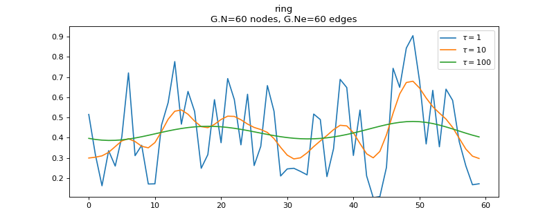
Create a bunch of smooth signals by low-pass filtering white noise:

>>> import matplotlib.pyplot as plt
>>> G = graphs.Ring(N=60)
>>> G.estimate_lmax()
>>> s = np.random.RandomState(42).uniform(size=(G.N, 10))
>>> taus = [1, 10, 100]
>>> s = filters.Heat(G, taus).filter(s)
>>> s.shape
(60, 10, 3)

Plot the 3 smoothed versions of the 10th signal:

>>> fig, ax = plt.subplots()
>>> G.set_coordinates('line1D')  # To visualize multiple signals in 1D.
>>> G.plot_signal(s[:, 9, :], ax=ax)
>>> legend = [r'$\tau={}$'.format(t) for t in taus]
>>> ax.legend(legend)  
<matplotlib.legend.Legend object at ...>

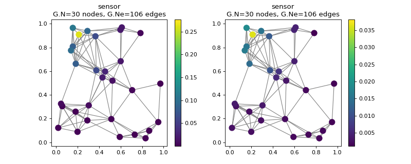
Low-pass filter a delta to create a localized smooth signal:

>>> G = graphs.Sensor(30, seed=42)
>>> G.compute_fourier_basis()  # Reproducible computation of lmax.
>>> s1 = np.zeros(G.N)
>>> s1[13] = 1
>>> s1 = filters.Heat(G, 3).filter(s1)
>>> s1.shape
(30,)

Filter and reconstruct our signal:

>>> g = filters.MexicanHat(G, Nf=4)
>>> s2 = g.analyze(s1)
>>> s2.shape
(30, 4)
>>> s2 = g.synthesize(s2)
>>> s2.shape
(30,)

Look how well we were able to reconstruct:

>>> fig, axes = plt.subplots(1, 2)
>>> G.plot_signal(s1, ax=axes[0])
>>> G.plot_signal(s2, ax=axes[1])
>>> print('{:.5f}'.format(np.linalg.norm(s1 - s2)))
0.29620

Perfect reconstruction with Itersine, a tight frame:

>>> g = filters.Itersine(G)
>>> s2 = g.analyze(s1, method='exact')
>>> s2 = g.synthesize(s2, method='exact')
>>> np.linalg.norm(s1 - s2) < 1e-10
True

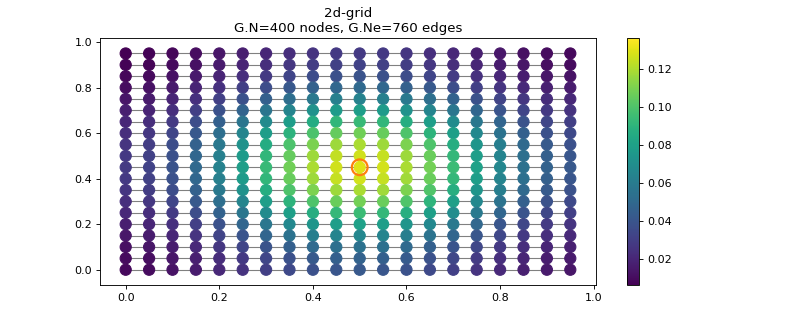
localize(i, **kwargs)[source]¶

Localize the kernels at a node (to visualize them).

That is particularly useful to visualize a filter in the vertex domain.

A kernel is localized by filtering a Kronecker delta, i.e.

\[\begin{split}g(L) s = g(L)_i, \text{ where } s_j = \delta_{ij} = \begin{cases} 0 \text{ if } i \neq j \\ 1 \text{ if } i = j \end{cases}\end{split}\]

Parameters:

i : int

Index of the node where to localize the kernel.

kwargs: dict

Parameters to be passed to the analyze() method.

Returns:

s : ndarray

Kernel localized at vertex i.

Examples

Visualize heat diffusion on a grid by localizing the heat kernel.

>>> import matplotlib
>>> N = 20
>>> DELTA = N//2 * (N+1)
>>> G = graphs.Grid2d(N)
>>> G.estimate_lmax()
>>> g = filters.Heat(G, 100)
>>> s = g.localize(DELTA)
>>> G.plot_signal(s, highlight=DELTA)

plot(**kwargs)[source]¶

Plot the filter bank’s frequency response.

See pygsp.plotting.plot_filter().

synthesize(s, method='chebyshev', order=30)[source]¶

Convenience wrapper around filter().

Will be an alias to adjoint().filter() in the future.

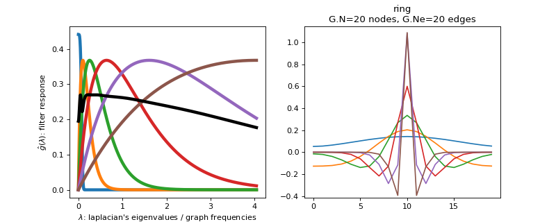
class pygsp.filters.Abspline(G, Nf=6, lpfactor=20, scales=None, **kwargs)[source]¶

Design an A B cubic spline wavelet filter bank.

Parameters:

G : graph

Nf : int

Number of filters from 0 to lmax (default = 6)

lpfactor : int

Low-pass factor lmin=lmax/lpfactor will be used to determine scales, the scaling function will be created to fill the lowpass gap. (default = 20)

scales : ndarray

Vector of scales to be used. By default, initialized with pygsp.utils.compute_log_scales().

Examples

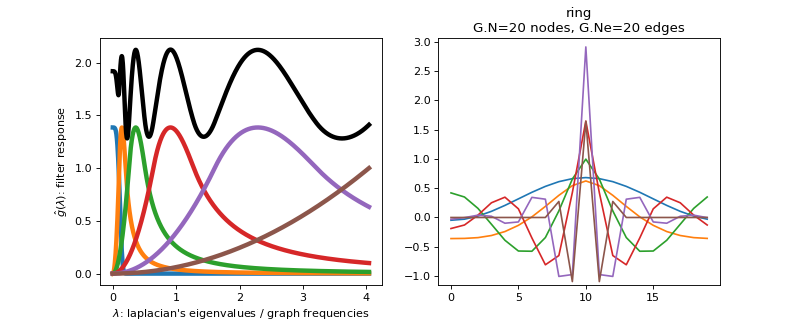
Filter bank’s representation in Fourier and time (ring graph) domains.

>>> import matplotlib.pyplot as plt
>>> G = graphs.Ring(N=20)
>>> G.estimate_lmax()
>>> G.set_coordinates('line1D')
>>> g = filters.Abspline(G)
>>> s = g.localize(G.N // 2)
>>> fig, axes = plt.subplots(1, 2)
>>> g.plot(ax=axes[0])
>>> G.plot_signal(s, ax=axes[1])

class pygsp.filters.Expwin(G, bmax=0.2, a=1.0, **kwargs)[source]¶

Design an exponential window filter.

Parameters:

G : graph

bmax : float

Maximum relative band (default = 0.2)

a : int

Slope parameter (default = 1)

Examples

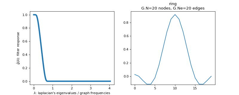
Filter bank’s representation in Fourier and time (ring graph) domains.

>>> import matplotlib.pyplot as plt
>>> G = graphs.Ring(N=20)
>>> G.estimate_lmax()
>>> G.set_coordinates('line1D')
>>> g = filters.Expwin(G)
>>> s = g.localize(G.N // 2)
>>> fig, axes = plt.subplots(1, 2)
>>> g.plot(ax=axes[0])
>>> G.plot_signal(s, ax=axes[1])

class pygsp.filters.Gabor(G, k)[source]¶

Design a Gabor filter bank.

Design a filter bank where the kernel k is placed at each graph frequency.

Parameters:

G : graph

k : lambda function

kernel

Examples

>>> G = graphs.Logo()
>>> k = lambda x: x / (1. - x)
>>> g = filters.Gabor(G, k);

class pygsp.filters.HalfCosine(G, Nf=6, **kwargs)[source]¶

Design an half cosine filter bank (tight frame).

Parameters:

G : graph

Nf : int

Number of filters from 0 to lmax (default = 6)

Examples

Filter bank’s representation in Fourier and time (ring graph) domains.

>>> import matplotlib.pyplot as plt
>>> G = graphs.Ring(N=20)
>>> G.estimate_lmax()
>>> G.set_coordinates('line1D')
>>> g = filters.HalfCosine(G)
>>> s = g.localize(G.N // 2)
>>> fig, axes = plt.subplots(1, 2)
>>> g.plot(ax=axes[0])
>>> G.plot_signal(s, ax=axes[1])

class pygsp.filters.Heat(G, tau=10, normalize=False, **kwargs)[source]¶

Design a filter bank of heat kernels.

The filter is defined in the spectral domain as

\[\hat{g}(x) = \exp \left( \frac{-\tau x}{\lambda_{\text{max}}} \right),\]

and is as such a low-pass filter. An application of this filter to a signal simulates heat diffusion.

Parameters:

G : graph

tau : int or list of ints

Scaling parameter. If a list, creates a filter bank with one filter per value of tau.

normalize : bool

Normalizes the kernel. Needs the eigenvalues.

Examples

Regular heat kernel.

>>> G = graphs.Logo()
>>> g = filters.Heat(G, tau=[5, 10])
>>> print('{} filters'.format(g.Nf))
2 filters
>>> y = g.evaluate(G.e)
>>> print('{:.2f}'.format(np.linalg.norm(y[0])))
9.76

Normalized heat kernel.

>>> g = filters.Heat(G, tau=[5, 10], normalize=True)
>>> y = g.evaluate(G.e)
>>> print('{:.2f}'.format(np.linalg.norm(y[0])))
1.00

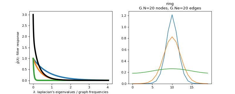
Filter bank’s representation in Fourier and time (ring graph) domains.

>>> import matplotlib.pyplot as plt
>>> G = graphs.Ring(N=20)
>>> G.estimate_lmax()
>>> G.set_coordinates('line1D')
>>> g = filters.Heat(G, tau=[5, 10, 100])
>>> s = g.localize(G.N // 2)
>>> fig, axes = plt.subplots(1, 2)
>>> g.plot(ax=axes[0])
>>> G.plot_signal(s, ax=axes[1])

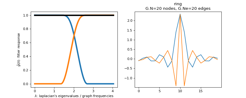
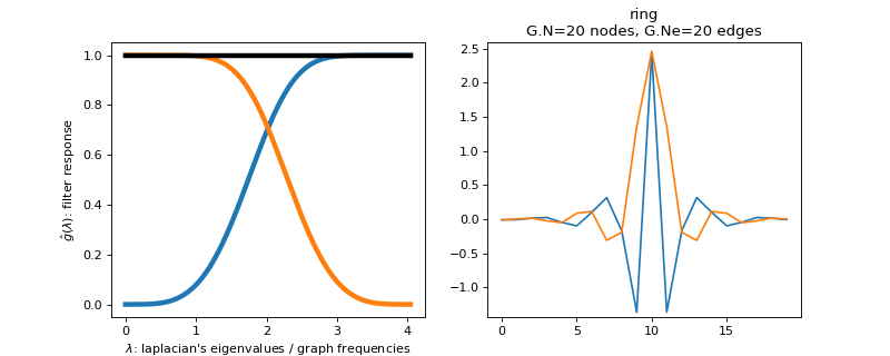
class pygsp.filters.Held(G, a=0.6666666666666666, **kwargs)[source]¶

Design 2 filters with the Held construction (tight frame).

This function create a parseval filterbank of \(2\) filters. The low-pass filter is defined by the function

\[\begin{split}f_{l}=\begin{cases} 1 & \mbox{if }x\leq a\\ \sin\left(2\pi\mu\left(\frac{x}{8a}\right)\right) & \mbox{if }a<x\leq2a\\ 0 & \mbox{if }x>2a \end{cases}\end{split}\]

with

\[\mu(x) = -1+24x-144*x^2+256*x^3\]

The high pass filter is adaptated to obtain a tight frame.

Parameters:

G : graph

a : float

See equation above for this parameter The spectrum is scaled between 0 and 2 (default = 2/3)

Examples

Filter bank’s representation in Fourier and time (ring graph) domains.

>>> import matplotlib.pyplot as plt
>>> G = graphs.Ring(N=20)
>>> G.estimate_lmax()
>>> G.set_coordinates('line1D')
>>> g = filters.Held(G)
>>> s = g.localize(G.N // 2)
>>> fig, axes = plt.subplots(1, 2)
>>> g.plot(ax=axes[0])
>>> G.plot_signal(s, ax=axes[1])

class pygsp.filters.Itersine(G, Nf=6, overlap=2.0, **kwargs)[source]¶

Design an itersine filter bank (tight frame).

Create an itersine half overlap filter bank of Nf filters. Going from 0 to lambda_max.

Parameters:

G : graph

Nf : int (optional)

Number of filters from 0 to lmax. (default = 6)

overlap : int (optional)

(default = 2)

Examples

Filter bank’s representation in Fourier and time (ring graph) domains.

>>> import matplotlib.pyplot as plt
>>> G = graphs.Ring(N=20)
>>> G.estimate_lmax()
>>> G.set_coordinates('line1D')
>>> g = filters.HalfCosine(G)
>>> s = g.localize(G.N // 2)
>>> fig, axes = plt.subplots(1, 2)
>>> g.plot(ax=axes[0])
>>> G.plot_signal(s, ax=axes[1])

class pygsp.filters.MexicanHat(G, Nf=6, lpfactor=20, scales=None, normalize=False, **kwargs)[source]¶

Design a filter bank of Mexican hat wavelets.

The Mexican hat wavelet is the second oder derivative of a Gaussian. Since we express the filter in the Fourier domain, we find:

\[\hat{g}_b(x) = x * \exp(-x)\]

for the band-pass filter. Note that in our convention the eigenvalues of the Laplacian are equivalent to the square of graph frequencies, i.e. \(x = \lambda^2\).

The low-pass filter is given by

Parameters:

G : graph

Nf : int

Number of filters to cover the interval [0, lmax].

lpfactor : int

Low-pass factor. lmin=lmax/lpfactor will be used to determine scales. The scaling function will be created to fill the low-pass gap.

scales : array-like

Scales to be used. By default, initialized with pygsp.utils.compute_log_scales().

normalize : bool

Whether to normalize the wavelet by the factor sqrt(scales).

Examples

Filter bank’s representation in Fourier and time (ring graph) domains.

>>> import matplotlib.pyplot as plt
>>> G = graphs.Ring(N=20)
>>> G.estimate_lmax()
>>> G.set_coordinates('line1D')
>>> g = filters.MexicanHat(G)
>>> s = g.localize(G.N // 2)
>>> fig, axes = plt.subplots(1, 2)
>>> g.plot(ax=axes[0])
>>> G.plot_signal(s, ax=axes[1])

class pygsp.filters.Meyer(G, Nf=6, scales=None, **kwargs)[source]¶

Design a filter bank of Meyer wavelets (tight frame).

Parameters:

G : graph

Nf : int

Number of filters from 0 to lmax (default = 6).

scales : ndarray

Vector of scales to be used (default: log scale).

References

Use of this kernel for SGWT proposed by Nora Leonardi and Dimitri Van De Ville in [LVDV11].

Examples

Filter bank’s representation in Fourier and time (ring graph) domains.

>>> import matplotlib.pyplot as plt
>>> G = graphs.Ring(N=20)
>>> G.estimate_lmax()
>>> G.set_coordinates('line1D')
>>> g = filters.Meyer(G)
>>> s = g.localize(G.N // 2)
>>> fig, axes = plt.subplots(1, 2)
>>> g.plot(ax=axes[0])
>>> G.plot_signal(s, ax=axes[1])

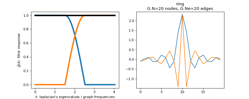
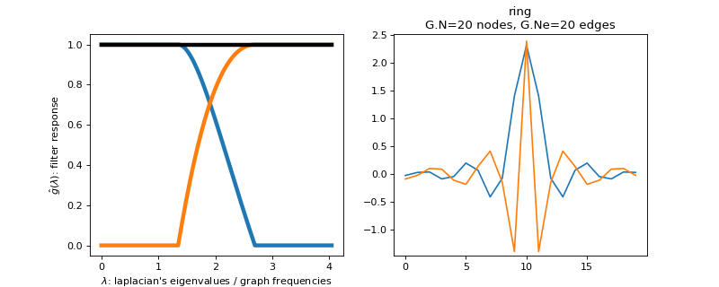
class pygsp.filters.Papadakis(G, a=0.75, **kwargs)[source]¶

Design 2 filters with the Papadakis construction (tight frame).

This function creates a Parseval filter bank of 2 filters. The low-pass filter is defined by the function

\[\begin{split}f_{l}=\begin{cases} 1 & \mbox{if }x\leq a\\ \sqrt{1-\frac{\sin\left(\frac{3\pi}{2a}x\right)}{2}} & \mbox{if }a<x\leq \frac{5a}{3} \\ 0 & \mbox{if }x>\frac{5a}{3} \end{cases}\end{split}\]

The high pass filter is adapted to obtain a tight frame.

Parameters:

G : graph

a : float

See above equation for this parameter. The spectrum is scaled between 0 and 2 (default = 3/4).

Examples

Filter bank’s representation in Fourier and time (ring graph) domains.

>>> import matplotlib.pyplot as plt
>>> G = graphs.Ring(N=20)
>>> G.estimate_lmax()
>>> G.set_coordinates('line1D')
>>> g = filters.Papadakis(G)
>>> s = g.localize(G.N // 2)
>>> fig, axes = plt.subplots(1, 2)
>>> g.plot(ax=axes[0])
>>> G.plot_signal(s, ax=axes[1])

class pygsp.filters.Regular(G, d=3, **kwargs)[source]¶

Design 2 filters with the regular construction (tight frame).

This function creates a Parseval filter bank of 2 filters. The low-pass filter is defined by a function \(f_l(x)\) between \(0\) and \(2\). For \(d = 0\).

\[f_{l}= \sin\left( \frac{\pi}{4} x \right)\]

For \(d = 1\)

\[f_{l}= \sin\left( \frac{\pi}{4} \left( 1+ \sin\left(\frac{\pi}{2}(x-1)\right) \right) \right)\]

For \(d = 2\)

\[f_{l}= \sin\left( \frac{\pi}{4} \left( 1+ \sin\left(\frac{\pi}{2} \sin\left(\frac{\pi}{2}(x-1)\right)\right) \right) \right)\]

And so forth for other degrees \(d\).

The high pass filter is adapted to obtain a tight frame.

Parameters:

G : graph

d : float

Degree (default = 3). See above equations.

Examples

Filter bank’s representation in Fourier and time (ring graph) domains.

>>> import matplotlib.pyplot as plt
>>> G = graphs.Ring(N=20)
>>> G.estimate_lmax()
>>> G.set_coordinates('line1D')
>>> g = filters.Regular(G)
>>> s = g.localize(G.N // 2)
>>> fig, axes = plt.subplots(1, 2)
>>> g.plot(ax=axes[0])
>>> G.plot_signal(s, ax=axes[1])

class pygsp.filters.Simoncelli(G, a=0.6666666666666666, **kwargs)[source]¶

Design 2 filters with the Simoncelli construction (tight frame).

This function creates a Parseval filter bank of 2 filters. The low-pass filter is defined by the function

\[\begin{split}f_{l}=\begin{cases} 1 & \mbox{if }x\leq a\\ \cos\left(\frac{\pi}{2}\frac{\log\left(\frac{x}{2}\right)}{\log(2)}\right) & \mbox{if }a<x\leq2a\\ 0 & \mbox{if }x>2a \end{cases}\end{split}\]

The high pass filter is adapted to obtain a tight frame.

Parameters:

G : graph

a : float

See above equation for this parameter. The spectrum is scaled between 0 and 2 (default = 2/3).

Examples

Filter bank’s representation in Fourier and time (ring graph) domains.

>>> import matplotlib.pyplot as plt
>>> G = graphs.Ring(N=20)
>>> G.estimate_lmax()
>>> G.set_coordinates('line1D')
>>> g = filters.Simoncelli(G)
>>> s = g.localize(G.N // 2)
>>> fig, axes = plt.subplots(1, 2)
>>> g.plot(ax=axes[0])
>>> G.plot_signal(s, ax=axes[1])

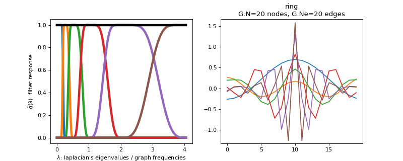
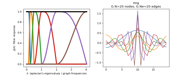
class pygsp.filters.SimpleTight(G, Nf=6, scales=None, **kwargs)[source]¶

Design a simple tight frame filter bank (tight frame).

These filters have been designed to be a simple tight frame wavelet filter bank. The kernel is similar to Meyer, but simpler. The function is essentially \(\sin^2(x)\) in ascending part and \(\cos^2\) in descending part.

Parameters:

G : graph

Nf : int

Number of filters to cover the interval [0, lmax].

scales : array-like

Scales to be used. Defaults to log scale.

Examples

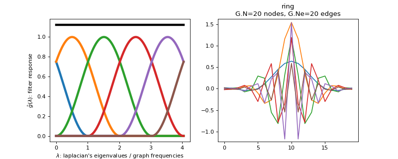
Filter bank’s representation in Fourier and time (ring graph) domains.

>>> import matplotlib.pyplot as plt
>>> G = graphs.Ring(N=20)
>>> G.estimate_lmax()
>>> G.set_coordinates('line1D')
>>> g = filters.SimpleTight(G)
>>> s = g.localize(G.N // 2)
>>> fig, axes = plt.subplots(1, 2)
>>> g.plot(ax=axes[0])
>>> G.plot_signal(s, ax=axes[1])

pygsp.filters.compute_cheby_coeff(f, m=30, N=None, *args, **kwargs)[source]¶

Compute Chebyshev coefficients for a Filterbank.

Parameters:

f : Filter

Filterbank with at least 1 filter

m : int

Maximum order of Chebyshev coeff to compute (default = 30)

N : int

Grid order used to compute quadrature (default = m + 1)

i : int

Index of the Filterbank element to compute (default = 0)

Returns:

c : ndarray

Matrix of Chebyshev coefficients

pygsp.filters.compute_jackson_cheby_coeff(filter_bounds, delta_lambda, m)[source]¶

To compute the m+1 coefficients of the polynomial approximation of an ideal band-pass between a and b, between a range of values defined by lambda_min and lambda_max.

Parameters:

filter_bounds : list

[a, b]

delta_lambda : list

[lambda_min, lambda_max]

m : int

Returns:

ch : ndarray

jch : ndarray

References

[TPGV16]

pygsp.filters.cheby_op(G, c, signal, **kwargs)[source]¶

Chebyshev polynomial of graph Laplacian applied to vector.

Parameters:

G : Graph

c : ndarray or list of ndarrays

Chebyshev coefficients for a Filter or a Filterbank

signal : ndarray

Signal to filter

Returns:

r : ndarray

Result of the filtering

pygsp.filters.cheby_rect(G, bounds, signal, **kwargs)[source]¶

Fast filtering using Chebyshev polynomial for a perfect rectangle filter.

Parameters:

G : Graph

bounds : array-like

The bounds of the pass-band filter

signal : array-like

Signal to filter

order : int (optional)

Order of the Chebyshev polynomial (default: 30)

Returns:

r : array-like

Result of the filtering

pygsp.filters.lanczos(A, order, x)[source]¶

TODO short description

Parameters:	A: ndarray

pygsp.filters.lanczos_op(f, s, order=30)[source]¶

Perform the lanczos approximation of the signal s.

Parameters:

f: Filter

s : ndarray

Signal to approximate.

order : int

Degree of the lanczos approximation. (default = 30)

Returns:

L : ndarray

lanczos approximation of s