Optimization problems: graph TV vs. Tikhonov regularization
Description
Modern signal processing often involves solving an optimization problem. Graph signal processing (GSP) consists roughly of working with linear operators defined by a graph (e.g., the graph Laplacian). The setting up of an optimization problem in the graph context is often then simply a matter of identifying which graph-defined linear operator is relevant to be used in a regularization and/or fidelity term.
This tutorial focuses on the problem of recovering a label signal on a graph from subsampled and noisy data, but most information should be fairly generally applied to other problems as well.
>>> import numpy as np
>>> from pygsp import graphs, plotting
>>>
>>> # Create a random sensor graph
>>> G = graphs.Sensor(N=256, distributed=True, seed=42)
>>> G.compute_fourier_basis()
>>>
>>> # Create label signal
>>> label_signal = np.copysign(np.ones(G.N), G.U[:, 3])
>>>
>>> fig, ax = G.plot(label_signal)
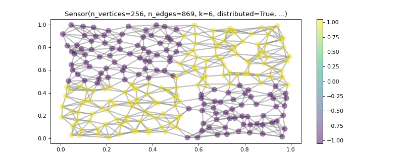
The first figure shows a plot of the original label signal, that we wish to recover, on the graph.
>>> rng = np.random.default_rng(42)
>>>
>>> # Create the mask
>>> M = rng.uniform(size=G.N)
>>> M = (M > 0.6).astype(float)  # Probability of having no label on a vertex.
>>>
>>> # Applying the mask to the data
>>> sigma = 0.1
>>> subsampled_noisy_label_signal = M * (label_signal + sigma * rng.standard_normal(G.N))
>>>
>>> fig, ax = G.plot(subsampled_noisy_label_signal)
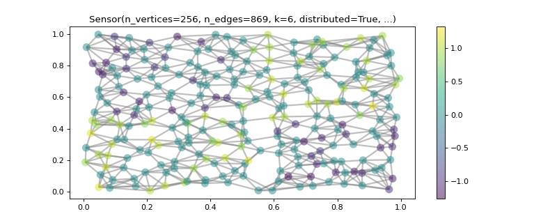
This figure shows the label signal on the graph after the application of the subsampling mask and the addition of noise. The label of more than half of the vertices has been set to \(0\).
Since the problem is ill-posed, we will use some regularization to reach a solution that is more in tune with what we expect a label signal to look like. We will compare two approaches, but they are both based on measuring local differences on the label signal. Those differences are essentially an edge signal: to each edge we can associate the difference between the label signals of its associated nodes. The linear operator that does such a mapping is called the graph gradient \(\nabla_G\), and, fortunately for us, it is available under the pygsp.graphs.Graph.D (for differential) attribute of any pygsp.graphs graph.
The reason for measuring local differences comes from prior knowledge: we assume label signals don’t vary too much locally. The precise measure of such variation is what distinguishes the two regularization approaches we’ll use.
The first one, shown below, is called graph total variation (TV) regularization. The quadratic fidelity term is multiplied by a regularization constant \(\gamma\) and its goal is to force the solution to stay close to the observed labels \(b\). The \(\ell_1\) norm of the action of the graph gradient is what’s called the graph TV. We will see that it promotes piecewise-constant solutions.
The second approach, called graph Tikhonov regularization, is to use a smooth (differentiable) quadratic regularizer. A consequence of this choice is that the solution will tend to have smoother transitions. The quadratic fidelity term is still the same.
Results and code
For solving the optimization problems we’ve assembled, you will need a numerical solver package. This part is implemented in this tutorial with the pyunlocbox, which is based on proximal splitting algorithms. Check also its documentation for more information about the parameters used here.
We start with the graph TV regularization. We will use the pyunlocbox.solvers.mlfbf solver from pyunlocbox. It is a primal-dual solver, which means for our problem that the regularization term will be written in terms of the dual variable \(u = \nabla_G x\), and the graph gradient \(\nabla_G\) will be passed to the solver as the primal-dual map. The value of \(3.0\) for the regularization parameter \(\gamma\) was chosen on the basis of the visual appeal of the returned solution.
>>> import pyunlocbox
>>>
>>> # Set the functions in the problem
>>> gamma = 3.0
>>> d = pyunlocbox.functions.dummy()
>>> r = pyunlocbox.functions.norm_l1()
>>> f = pyunlocbox.functions.norm_l2(w=M, y=subsampled_noisy_label_signal,
...                                  lambda_=gamma)
>>>
>>> # Define the solver
>>> G.compute_differential_operator()
>>> L = G.D.T.toarray()
>>> step = 0.999 / (1 + np.linalg.norm(L))
>>> solver = pyunlocbox.solvers.mlfbf(L=L, step=step)
>>>
>>> # Solve the problem
>>> x0 = subsampled_noisy_label_signal.copy()
>>> prob1 = pyunlocbox.solvers.solve([d, r, f], solver=solver,
...                                  x0=x0, rtol=0, maxit=1000)
Solution found after 1000 iterations:
    objective function f(sol) = 2.213139e+02
    stopping criterion: MAXIT
>>>
>>> fig, ax = G.plot(prob1['sol'])
This figure shows the label signal recovered by graph total variation regularization. We can confirm here that this sort of regularization does indeed promote piecewise-constant solutions.
>>> # Set the functions in the problem
>>> r = pyunlocbox.functions.norm_l2(A=L, tight=False)
>>>
>>> # Define the solver
>>> step = 0.999 / np.linalg.norm(np.dot(L.T, L) + gamma * np.diag(M), 2)
>>> solver = pyunlocbox.solvers.gradient_descent(step=step)
>>>
>>> # Solve the problem
>>> x0 = subsampled_noisy_label_signal.copy()
>>> prob2 = pyunlocbox.solvers.solve([r, f], solver=solver,
...                                  x0=x0, rtol=0, maxit=1000)
Solution found after 1000 iterations:
    objective function f(sol) = 6.422673e+01
    stopping criterion: MAXIT
>>>
>>> fig, ax = G.plot(prob2['sol'])
This last figure shows the label signal recovered by Tikhonov regularization. As expected, the recovered label signal has smoother transitions than the one obtained by graph TV regularization.