Learning

The pygsp.learning module provides functions to solve learning problems.

Semi-supervized learning

Those functions help to solve a semi-supervized learning problem, i.e., a problem where only some values of a graph signal are known and the others shall be inferred.

regression_tikhonov(G, y, M[, tau])	Solve a regression problem on graph via Tikhonov minimization.
classification_tikhonov(G, y, M[, tau])	Solve a classification problem on graph via Tikhonov minimization.
classification_tikhonov_simplex(G, y, M[, tau])	Solve a classification problem on graph via Tikhonov minimization with simple constraints.

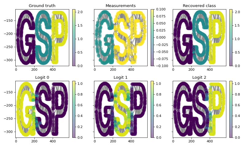
pygsp.learning.classification_tikhonov(G, y, M, tau=0)

Solve a classification problem on graph via Tikhonov minimization.

The function first transforms \(y\) in logits \(Y\), then solves

\[\operatorname*{arg min}_X \| M X - Y \|_2^2 + \tau \ tr(X^T L X)\]

if \(\tau > 0\), and

\[\operatorname*{arg min}_X tr(X^T L X) \ \text{ s. t. } \ Y = M X\]

otherwise, where \(X\) and \(Y\) are logits. The function returns the maximum of the logits.

Parameters

Gpygsp.graphs.Graph

yarray, length G.n_vertices

Measurements.

Marray of boolean, length G.n_vertices

Masking vector.

taufloat

Regularization parameter.

Returns

logitsarray, length G.n_vertices

The logits \(X\).

Examples

>>> from pygsp import graphs, learning
>>> import matplotlib.pyplot as plt
>>>
>>> G = graphs.Logo()

Create a ground truth signal:

>>> signal = np.zeros(G.n_vertices)
>>> signal[G.info['idx_s']] = 1
>>> signal[G.info['idx_p']] = 2

Construct a measurement signal from a binary mask:

>>> rng = np.random.default_rng(42)
>>> mask = rng.uniform(0, 1, G.n_vertices) > 0.5
>>> measures = signal.copy()
>>> measures[~mask] = np.nan

Solve the classification problem by reconstructing the signal:

>>> recovery = learning.classification_tikhonov(G, measures, mask, tau=0)

Plot the results. Note that we recover the class with np.argmax(recovery, axis=1).

>>> prediction = np.argmax(recovery, axis=1)
>>> fig, ax = plt.subplots(2, 3, sharey=True, figsize=(10, 6))
>>> _ = G.plot(signal, ax=ax[0, 0], title='Ground truth')
>>> _ = G.plot(measures, ax=ax[0, 1], title='Measurements')
>>> _ = G.plot(prediction, ax=ax[0, 2], title='Recovered class')
>>> _ = G.plot(recovery[:, 0], ax=ax[1, 0], title='Logit 0')
>>> _ = G.plot(recovery[:, 1], ax=ax[1, 1], title='Logit 1')
>>> _ = G.plot(recovery[:, 2], ax=ax[1, 2], title='Logit 2')
>>> _ = fig.tight_layout()

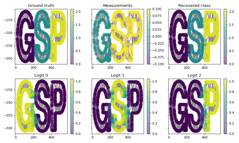
pygsp.learning.classification_tikhonov_simplex(G, y, M, tau=0.1, **kwargs)

Solve a classification problem on graph via Tikhonov minimization with simple constraints.

The function first transforms \(y\) in logits \(Y\), then solves

\[\operatorname*{arg min}_X \| M X - Y \|_2^2 + \tau \ tr(X^T L X) \text{ s.t. } sum(X) = 1 \text{ and } X >= 0,\]

where \(X\) and \(Y\) are logits.

Parameters

Gpygsp.graphs.Graph

yarray, length G.n_vertices

Measurements.

Marray of boolean, length G.n_vertices

Masking vector.

taufloat

Regularization parameter.

kwargsdict

Parameters for pyunlocbox.solvers.solve().

Returns

logitsarray, length G.n_vertices

The logits \(X\).

Examples

>>> from pygsp import graphs, learning
>>> import matplotlib.pyplot as plt
>>>
>>> G = graphs.Logo()
>>> G.estimate_lmax()

Create a ground truth signal:

>>> signal = np.zeros(G.n_vertices)
>>> signal[G.info['idx_s']] = 1
>>> signal[G.info['idx_p']] = 2

Construct a measurement signal from a binary mask:

>>> rng = np.random.default_rng(42)
>>> mask = rng.uniform(0, 1, G.n_vertices) > 0.5
>>> measures = signal.copy()
>>> measures[~mask] = np.nan

Solve the classification problem by reconstructing the signal:

>>> recovery = learning.classification_tikhonov_simplex(
...     G, measures, mask, tau=0.1, verbosity='NONE')

Plot the results. Note that we recover the class with np.argmax(recovery, axis=1).

>>> prediction = np.argmax(recovery, axis=1)
>>> fig, ax = plt.subplots(2, 3, sharey=True, figsize=(10, 6))
>>> _ = G.plot(signal, ax=ax[0, 0], title='Ground truth')
>>> _ = G.plot(measures, ax=ax[0, 1], title='Measurements')
>>> _ = G.plot(prediction, ax=ax[0, 2], title='Recovered class')
>>> _ = G.plot(recovery[:, 0], ax=ax[1, 0], title='Logit 0')
>>> _ = G.plot(recovery[:, 1], ax=ax[1, 1], title='Logit 1')
>>> _ = G.plot(recovery[:, 2], ax=ax[1, 2], title='Logit 2')
>>> _ = fig.tight_layout()

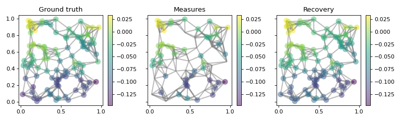
pygsp.learning.regression_tikhonov(G, y, M, tau=0)

Solve a regression problem on graph via Tikhonov minimization.

The function solves

\[\operatorname*{arg min}_x \| M x - y \|_2^2 + \tau \ x^T L x\]

if \(\tau > 0\), and

\[\operatorname*{arg min}_x x^T L x \ \text{ s. t. } \ y = M x\]

otherwise.

Parameters

Gpygsp.graphs.Graph

yarray, length G.n_vertices

Measurements.

Marray of boolean, length G.n_vertices

Masking vector.

taufloat

Regularization parameter.

Returns

xarray, length G.n_vertices

Recovered values \(x\).

Examples

>>> from pygsp import graphs, filters, learning
>>> import matplotlib.pyplot as plt
>>>
>>> G = graphs.Sensor(N=100, seed=42)
>>> G.estimate_lmax()

Create a smooth ground truth signal:

>>> filt = lambda x: 1 / (1 + 10*x)
>>> filt = filters.Filter(G, filt)
>>> rng = np.random.default_rng(42)
>>> signal = filt.analyze(rng.normal(size=G.n_vertices))

Construct a measurement signal from a binary mask:

>>> mask = rng.uniform(0, 1, G.n_vertices) > 0.5
>>> measures = signal.copy()
>>> measures[~mask] = np.nan

Solve the regression problem by reconstructing the signal:

>>> recovery = learning.regression_tikhonov(G, measures, mask, tau=0)

Plot the results:

>>> fig, (ax1, ax2, ax3) = plt.subplots(1, 3, sharey=True, figsize=(10, 3))
>>> limits = [signal.min(), signal.max()]
>>> _ = G.plot(signal, ax=ax1, limits=limits, title='Ground truth')
>>> _ = G.plot(measures, ax=ax2, limits=limits, title='Measures')
>>> _ = G.plot(recovery, ax=ax3, limits=limits, title='Recovery')
>>> _ = fig.tight_layout()