Introduction to the PyGSP
This tutorial will show you the basic operations of the toolbox. After installing the package with pip, start by opening a python shell, e.g. a Jupyter notebook, and import the PyGSP. We will also need NumPy to create matrices and arrays.
>>> import numpy as np
>>> import matplotlib.pyplot as plt
>>> from pygsp import graphs, filters, plotting
We then set default plotting parameters. We’re using the matplotlib backend
to embed plots in this tutorial. The pyqtgraph backend is best suited for
interactive visualization.
>>> plotting.BACKEND = 'matplotlib'
>>> plt.rcParams['figure.figsize'] = (10, 5)
Graphs
Most likely, the first thing you would like to do is to create a graph. In this toolbox, a graph is encoded as an adjacency, or weight, matrix. That is because it’s the most efficient representation to deal with when using spectral methods. As such, you can construct a graph from any adjacency matrix as follows.
>>> rng = np.random.default_rng(1)  # Reproducible results.
>>> W = rng.uniform(size=(30, 30))  # Full graph.
>>> W[W < 0.93] = 0  # Sparse graph.
>>> W = W + W.T  # Symmetric graph.
>>> np.fill_diagonal(W, 0)  # No self-loops.
>>> G = graphs.Graph(W)
>>> print('{} nodes, {} edges'.format(G.N, G.Ne))
30 nodes, 64 edges
The pygsp.graphs.Graph class we just instantiated is the base class
for all graph objects, which offers many methods and attributes.
Given, a graph object, we can test some properties.
>>> G.is_connected()
True
>>> G.is_directed()
False
We can retrieve our weight matrix, which is stored in a sparse format.
>>> (G.W == W).all()
True
>>> type(G.W)
<class 'scipy.sparse.csr.csr_matrix'>
We can access the graph Laplacian
>>> # The graph Laplacian (combinatorial by default).
>>> G.L.shape
(30, 30)
We can also compute and get the graph Fourier basis (see below).
>>> G.compute_fourier_basis()
>>> G.U.shape
(30, 30)
Or the graph differential operator, useful to e.g. compute the gradient or smoothness of a signal.
>>> G.compute_differential_operator()
>>> G.D.shape
(30, 64)
Note
Note that we called pygsp.graphs.Graph.compute_fourier_basis() and
pygsp.graphs.Graph.compute_differential_operator() before accessing
the Fourier basis pygsp.graphs.Graph.U and the differential
operator pygsp.graphs.Graph.D. Doing so is however not mandatory as
those matrices would have been computed when requested (lazy evaluation).
Omitting to call the compute functions does print a warning to tell you
that a potentially heavy computation is taking place under the hood (that’s
also the reason those matrices are not computed when the graph object is
instantiated). It is thus encouraged to call them so that you are aware of
the involved computations.
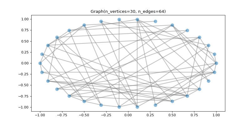
To be able to plot a graph, we need to embed its nodes in a 2D or 3D space.
While most included graph models define these coordinates, the graph we just
created do not. We only passed a weight matrix after all. Let’s set some
coordinates with pygsp.graphs.Graph.set_coordinates() and plot our graph.
>>> G.set_coordinates('ring2D')
>>> fig, ax = G.plot()
While we created our first graph ourselves, many standard models of graphs are
implemented as subclasses of the Graph class and can be easily instantiated.
Check the pygsp.graphs module to get a list of them and learn more about
the Graph object.
Fourier basis
As in classical signal processing, the Fourier transform plays a central role
in graph signal processing. Getting the Fourier basis is however
computationally intensive as it needs to fully diagonalize the Laplacian. While
it can be used to filter signals on graphs, a better alternative is to use one
of the fast approximations (see pygsp.filters.Filter.filter()). Let’s
compute it nonetheless to visualize the eigenvectors of the Laplacian.
Analogous to classical Fourier analysis, they look like sinuses on the graph.
Let’s plot the second and third eigenvectors (the first is constant). Those are
graph signals, i.e. functions \(s: \mathcal{V} \rightarrow \mathbb{R}^d\)
which assign a set of values (a vector in \(\mathbb{R}^d\)) at every node
\(v \in \mathcal{V}\) of the graph.
>>> G = graphs.Logo()
>>> G.compute_fourier_basis()
>>>
>>> fig, axes = plt.subplots(1, 2, figsize=(10, 3))
>>> for i, ax in enumerate(axes):
...     _ = G.plot(G.U[:, i+1], vertex_size=30, ax=ax)
...     _ = ax.set_title('Eigenvector {}'.format(i+2))
...     ax.set_axis_off()
>>> fig.tight_layout()

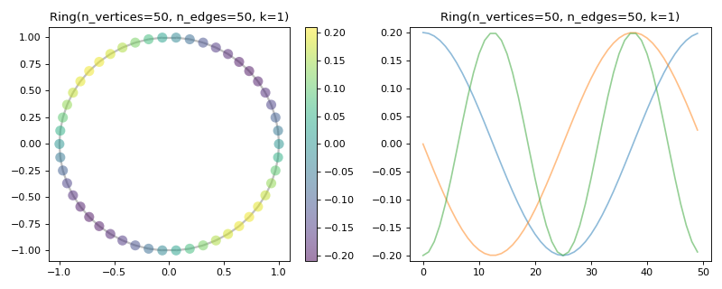
The parallel with classical signal processing is best seen on a ring graph, where the graph Fourier basis is equivalent to the classical Fourier basis. The following plot shows some eigenvectors drawn on a 1D and 2D embedding of the ring graph. While the signals are easier to interpret on a 1D plot, the 2D plot best represents the graph.
>>> G2 = graphs.Ring(N=50)
>>> G2.compute_fourier_basis()
>>> fig, axes = plt.subplots(1, 2, figsize=(10, 4))
>>> _ = G2.plot(G2.U[:, 4], ax=axes[0])
>>> G2.set_coordinates('line1D')
>>> _ = G2.plot(G2.U[:, 1:4], ax=axes[1])
>>> fig.tight_layout()
Filters
To filter signals on graphs, we need to define filters. They are represented in
the toolbox by the pygsp.filters.Filter class. Filters are usually
defined in the spectral domain. Given the transfer function
let’s define and plot that low-pass filter:
>>> tau = 1
>>> def g(x):
...     return 1. / (1. + tau * x)
>>> g = filters.Filter(G, g)
>>>
>>> fig, ax = g.plot(eigenvalues=True, title='Filter frequency response')
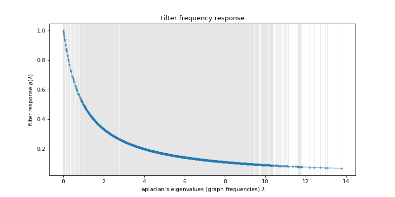
The filter is plotted along all the spectrum of the graph. The black crosses are the eigenvalues of the Laplacian. They are the points where the continuous filter will be evaluated to create a discrete filter.
Note
You can put multiple functions in a list to define a filter bank!
Note
The pygsp.filters module implements various standard filters.
Let’s create a graph signal and add some random noise.
>>> # Graph signal: each letter gets a different value + additive noise.
>>> s = np.zeros(G.N)
>>> s[G.info['idx_g']] = -1
>>> s[G.info['idx_s']] = 0
>>> s[G.info['idx_p']] = 1
>>> s += rng.uniform(-0.5, 0.5, size=G.N)
We can now try to denoise that signal by filtering it with the above defined low-pass filter.
>>> s2 = g.filter(s)
>>>
>>> fig, axes = plt.subplots(1, 2, figsize=(10, 3))
>>> _ = G.plot(s, vertex_size=30, title='noisy', ax=axes[0])
>>> axes[0].set_axis_off()
>>> _ = G.plot(s2, vertex_size=30, title='cleaned', ax=axes[1])
>>> axes[1].set_axis_off()
>>> fig.tight_layout()
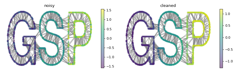
While the noise is largely removed thanks to the filter, some energy is diffused between the letters. This is the typical behavior of a low-pass filter.
So here are the basics for the PyGSP. Please check the other tutorials and the reference guide for more. Enjoy!
Note
Please see the review article The Emerging Field of Signal Processing on Graphs: Extending High-Dimensional Data Analysis to Networks and Other Irregular Domains for an overview of the methods this package leverages.